Unit 4 · 8 teaching hours · 19 min read
Decision Support, Business Intelligence and Knowledge Management
What the syllabus asks for 8
- The decision-making process
- Decision tables
- Decisions under risk: payoff tables and EMV
- Decisions under uncertainty (probabilities unknown)
- Decision trees and the value of a pilot
- Business intelligence and data warehousing
- Knowledge management
- Seeing decisions: steps, payoffs, trees and warehouses
Choosing between buying a server, renting cloud capacity or doing nothing is a decision under uncertainty: nobody knows next year's demand.
A good manager does not guess; she lists the alternatives, the possible futures and what each alternative earns in each future, assigns probabilities, and computes the expected result.
This unit gives the structured tools for that: decision tables (to make rule-based decisions complete and consistent), payoff tables with expected monetary value, regret and other criteria for decisions where probabilities are unknown, decision trees, and the business intelligence and knowledge systems that feed them.
- Simon's decision process; DSS architecture.
- Decision tables with a completeness check; payoff tables, EMV, EVPI and four uncertainty criteria.
- Decision trees and the value of a pilot study.
- Data warehouses, OLAP, KPIs and dashboards; knowledge management (SECI).
4.1 The decision-making process
Herbert Simon's model has four phases: intelligence (find and define the problem), design (develop alternatives and a model), choice (select the best alternative) and implementation (carry it out and monitor).
A DSS supports each: queries and dashboards for intelligence, models and what-if analysis for design, optimisation and ranking for choice, and tracking for implementation.
Decisions can be made under certainty (outcomes known), under risk (outcomes uncertain but probabilities known), or under uncertainty (probabilities unknown). The rest of the unit treats the last two.
4.2 Decision tables
For rule-based decisions with several conditions, a decision table lists conditions above the line and actions below, with one column per rule.
It is more compact than prose and easy to test for completeness (every combination covered) and consistency (no combination gets two different actions). A dash (—) means "don't care".
Conditions: existing customer, holds a salary account, requested amount at most 5× monthly salary.
| Condition / action | R1 | R2 | R3 | R4 | R5 |
|---|---|---|---|---|---|
| Existing customer | Y | Y | Y | N | N |
| Salary account | Y | Y | N | — | — |
| Amount ≤ 5× salary | Y | N | — | Y | N |
| Action | Approve | Refer to manager | Refer to manager | Refer to manager | Reject |
Three conditions give 2³ = 8 combinations. Expanding the don't-cares gives the full table below; every combination matches exactly one rule, so the table is complete and consistent.
| Customer | Salary a/c | ≤ 5× salary | Matching rule | Action |
|---|---|---|---|---|
| Y | Y | Y | R1 | Approve |
| Y | Y | N | R2 | Refer to manager |
| Y | N | Y | R3 | Refer to manager |
| Y | N | N | R3 | Refer to manager |
| N | Y | Y | R4 | Refer to manager |
| N | Y | N | R5 | Reject |
| N | N | Y | R4 | Refer to manager |
| N | N | N | R5 | Reject |
If a combination matched no rule the table would be incomplete, and if it matched rules with different actions it would be contradictory. Tools enumerate the 2ⁿ combinations to check this automatically, as was done for the table above.
A table with n conditions can be reduced by merging rules that differ in only one condition and share an action (consolidation).
4.3 Decisions under risk: payoff tables and EMV
A payoff table shows the profit (or cost) of each alternative in each state of nature. With probabilities, the expected monetary value (EMV) of an alternative is the probability-weighted average: EMV = Σ pⱼ × payoffⱼ.
States: high demand (p = 0.3), medium (0.5), low (0.2). Payoffs in Rs '000 over the first year:
| Alternative (Rs '000 profit) | High demand | Medium | Low | EMV |
|---|---|---|---|---|
| Large on-premise server | 900 | 400 | -300 | 410 |
| Cloud, auto-scaling | 700 | 450 | 100 | 455 |
| Small server | 300 | 250 | 150 | 245 |
The best EMV is Cloud, auto-scaling at Rs 455 thousand. Note the large on-premise server has the highest possible payoff (900) but also the worst loss (−300): EMV ignores your attitude to risk.
Expected value of perfect information (EVPI). Suppose a forecaster could tell you the state in advance.
You would pick the best action in each state: expected profit with perfect information = 0.3 × 900 + 0.5 × 450 + 0.2 × 150 = Rs 525 thousand. EVPI = 525 − 455 = Rs 70 thousand.
No market study that costs more than this can be worth buying; it is the ceiling on the value of any information.
4.4 Decisions under uncertainty (probabilities unknown)
When probabilities cannot be estimated, several criteria express different attitudes. Using the same payoffs:
- Maximin (pessimist): choose the alternative with the best worst-case. Worst cases are −300, 100 and 150, so the choice is Small server (guaranteeing 150).
- Maximax (optimist): choose the best best-case: the large server (900).
- Laplace (equal likelihood): average the payoffs, assuming all states equally likely; best is Cloud, auto-scaling with 416.7.
- Hurwicz (coefficient of optimism α = 0.6): α × best + (1 − α) × worst: Large on-premise server = 420, Cloud, auto-scaling = 460, Small server = 240; best is Cloud, auto-scaling.
- Minimax regret (Savage): regret = best payoff in that state minus this alternative's payoff; choose the smallest maximum regret.
| Alternative (regret, Rs '000) | High demand | Medium | Low | Maximum regret |
|---|---|---|---|---|
| Large on-premise server | 0 | 50 | 450 | 450 |
| Cloud, auto-scaling | 200 | 0 | 50 | 200 |
| Small server | 600 | 200 | 0 | 600 |
Minimax regret selects Cloud, auto-scaling (maximum regret 200). Different criteria can pick different alternatives; the manager must choose the criterion that matches the organisation's attitude to risk before seeing the numbers.
4.5 Decision trees and the value of a pilot
A decision tree draws decisions as squares, chance events as circles and payoffs at the leaves. It is solved by rolling back: at chance nodes take the expected value, at decision nodes take the best branch.
A full roll-out costs nothing extra to decide but pays Rs 800 thousand if successful (probability 0.6) and loses Rs 300 thousand if not. Build now has EMV = 0.6 × 800 + 0.4 × (−300) = 360.
Alternatively, a pilot costing Rs 50 thousand gives a "good" result with probability 0.5 and a "bad" one with 0.5. After a good pilot the probability of success rises to 0.9, after a bad one it falls to 0.3 (consistent with 0.5 × 0.9 + 0.5 × 0.3 = 0.6). Rolling back:
- After "good": EMV(roll out) = 0.9 × 800 + 0.1 × (−300) = 690; roll out.
- After "bad": EMV(roll out) = 0.3 × 800 + 0.7 × (−300) = 30, which is still above 0, so roll out anyway (30).
- Expected before the pilot cost: 0.5 × 690 + 0.5 × 30 = 360; minus the 50 cost gives 310.
The better choice is build now, by -50. The pilot changes no decision (we would roll out in both cases), so its information has zero value and its cost is wasted. A pilot is worth buying only if some outcome would make you not proceed.
4.6 Business intelligence and data warehousing
Business intelligence (BI) is the set of technologies for turning data into insight.
Operational databases are optimised for fast transactions (OLTP) and are poor for analysis, so a data warehouse copies, cleans and integrates data from many sources into a subject-oriented, time-variant, non-volatile store optimised for queries.
The pipeline is ETL: extract from source systems, transform (clean, convert codes, aggregate), load into the warehouse.
Data are often arranged as a star schema: a central fact table (sales amounts) linked to dimension tables (date, product, branch, customer).
OLAP (online analytical processing) lets users slice, dice, drill down and roll up through these dimensions: total sales by province, then by district, then by branch; the same by quarter instead of year.
Data mining finds patterns automatically (market-basket analysis: customers who buy noodles buy cooking oil; classification; clustering; anomaly detection). A data mart is a department-sized warehouse.
KPIs and dashboards. A good KPI is measurable, tied to a goal, and has an owner and a target: non-performing loan ratio, order fulfilment time, customer churn, system uptime.
A dashboard shows few KPIs, with comparison against target and colour-coded status. Avoid vanity metrics (page views without conversions).
4.7 Knowledge management
Knowledge management (KM) is the set of practices for creating, capturing, sharing and using knowledge. Nonaka and Takeuchi's SECI model describes four conversions between tacit and explicit knowledge:
| Mode | Conversion | Example |
|---|---|---|
| Socialisation | Tacit → tacit | Apprenticeship; a new engineer shadowing a senior |
| Externalisation | Tacit → explicit | Writing a post-incident review |
| Combination | Explicit → explicit | Merging reports into a policy handbook |
| Internalisation | Explicit → tacit | Learning by working through the handbook |
Technology supports KM through document repositories, wikis, expert directories, communities of practice and search; but culture (willingness to share, recognition for contributors) decides whether it works.
Geographic information systems (GIS) and expert systems are special DSS: a GIS analyses location data (flood risk by ward), while an expert system encodes expert rules for tasks such as diagnosis.
Artificial intelligence now adds recommendation, forecasting and natural-language assistants to BI.
4.8 Seeing decisions: steps, payoffs, trees and warehouses
Decision methods are numerical, so each comes with a picture.
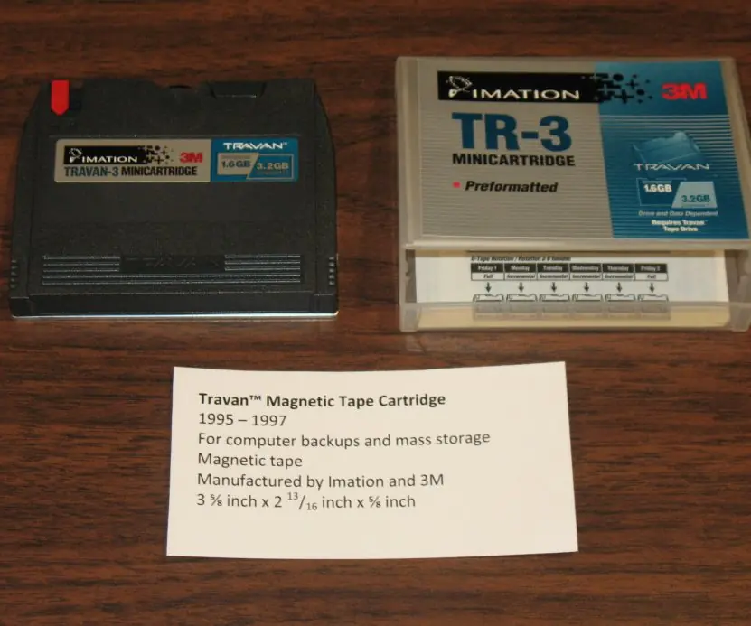
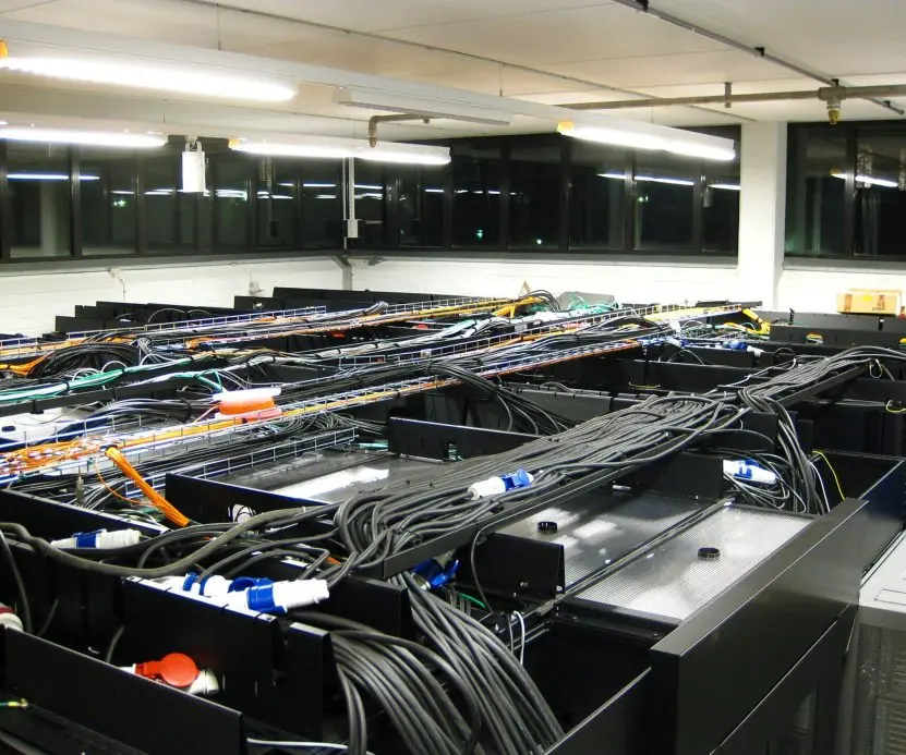
The plate shows the physical memory of business intelligence, from an old backup tape to a server hall, and the figures show the decision process, the payoff comparison of Section 4.3, the roll-back of the decision tree in Section 4.5 and the path of data into a data warehouse.


4.8.1 Eight uses of business intelligence in Nepali organisations
- Sales analysis. A retail chain studies sales by product, branch and week to see what sells and what does not. Weak items can be dropped and fast items kept in stock. A supermarket in Lalitpur can decide the festival-season order from last year's pattern.
- Customer segmentation. A bank groups customers by age, balance and use of services. Each group gets suitable products and offers. A youth savings account for students and a remittance account for families of migrant workers are examples.
- Fraud detection. Unusual patterns, such as many withdrawals in different cities within an hour, are flagged for checking. Rules and models run on the warehouse and the live feed. This protects customers and reduces the loss of the bank.
- Credit risk assessment. Past repayment history is analysed to predict who will default. Loan officers use the score together with their own judgement. A better score model means fewer bad loans and fairer access to credit.
- Operations planning. A telecom operator studies call traffic by hour and place to decide where to add capacity. A hydropower company studies demand to plan maintenance. Decisions follow the data and not only experience.
- Education analytics. A university studies attendance, internal marks and results to find students at risk. Teachers can offer help early. Tribhuvan University style examination data, when well kept, shows which subjects have the highest failure.
- Performance dashboards. Executives see sales, cash, complaints and targets on one screen with colour signals. They need not wait for monthly paper reports. Problems are noticed within days.
- Forecasting and budgeting. Trends in the warehouse are used to forecast demand, revenue and cost. A budget based on three years of data is more reliable than a guess. Forecast errors are measured and used to improve the next forecast.
Chapter summary
- Decisions follow intelligence, design, choice and implementation; DSS support each phase.
- Decision tables expose missing or contradictory rules; 2ⁿ combinations must each match exactly one rule.
- Under risk use EMV; EVPI bounds the value of information. Under uncertainty use maximin, maximax, Laplace, Hurwicz or minimax regret, chosen to fit the risk attitude.
- Decision trees are solved by rolling back; information is valuable only if it can change the decision.
- BI relies on ETL, warehouses, star schemas, OLAP and KPIs; KM converts tacit and explicit knowledge (SECI).
Practice
- List Simon's four phases and the DSS support for each.
- How many rules does a complete decision table with 4 yes/no conditions need before consolidation?
- Compute the EMV of the small server in the payoff table.
- Compute EVPI from the figures given in section 4.3.
- Which alternative does maximin choose and why might a risk-averse owner like it?
- What do OLTP and OLAP optimise for?
- Explain ETL in three steps.
- Give one example for each SECI mode.
- Why was the pilot not worth Rs 50 thousand in the tree example?
- Name four properties of a good KPI.
Answers and worked solutions
1. Intelligence (queries, dashboards), design (models, what-if), choice (optimisation, ranking), implementation (tracking, alerts).
2. 2⁴ = 16.
3. 0.3 × 300 + 0.5 × 250 + 0.2 × 150 = 90 + 125 + 30 = 245 (Rs '000).
4. 525 − 455 = 70 (Rs '000).
5. Small server (worst case +150). It guarantees a profit whatever happens.
6. OLTP: fast, many small updates and lookups. OLAP: complex read queries over large historical data.
7. Extract data from sources, transform it (clean, standardise, aggregate), load it into the warehouse.
8. Socialisation: shadowing. Externalisation: writing a procedure from experience. Combination: compiling reports into one manual. Internalisation: learning by practising a manual.
9. Roll-out has a positive EMV even after a bad pilot, so the decision never changes; the information has zero value.
10. Measurable, linked to a goal, has an owner, has a target and a time frame (also timely and understandable).
Model answers: medium (5 marks) and long (10 marks) questions
Q1 (5 marks). Explain EMV and EVPI. For the hosting table (probabilities 0.3, 0.5, 0.2) calculate the EMV of each option, choose the best and find the EVPI.
Introduction. When the probabilities of the states of nature are known, the expected monetary value (EMV) of an alternative is the probability-weighted average of its payoffs (section 4.3, Figure 4.2).
- Large server. 0.3 x 900 + 0.5 x 400 + 0.2 x (-300) = 270 + 200 - 60 = 410.
- Cloud, auto-scaling. 0.3 x 700 + 0.5 x 450 + 0.2 x 100 = 210 + 225 + 20 = 455.
- Small server. 0.3 x 300 + 0.5 x 250 + 0.2 x 150 = 90 + 125 + 30 = 245 (all in Rs thousand).
- Best choice. The cloud option, with the highest EMV of Rs 455 thousand.
- EVPI. With perfect information we pick the best action in each state: 0.3 x 900 + 0.5 x 450 + 0.2 x 150 = 270 + 225 + 30 = 525. EVPI = 525 - 455 = Rs 70 thousand, the maximum we should pay for a forecast.
- Limitation. EMV ignores risk attitude: the large server has the best top payoff (900) but also the worst loss (-300).
| Option | High 0.3 | Medium 0.5 | Low 0.2 | EMV |
|---|---|---|---|---|
| Large server | 900 | 400 | -300 | 410 |
| Cloud | 700 | 450 | 100 | 455 |
| Small server | 300 | 250 | 150 | 245 |
Conclusion. The cloud option is chosen on EMV, and no forecast is worth more than Rs 70 thousand.
Q2 (5 marks). Draw and solve the decision tree: build now (success 0.6 gives +800, failure 0.4 gives -300) or pilot first (cost 50, good result 0.5 raises success to 0.9, bad result lowers it to 0.3).
Introduction. A decision tree shows decisions as squares, chance events as circles and payoffs at the leaves, and is solved by rolling back from the right (section 4.5, Figure 4.3).
- Build now. 0.6 x 800 + 0.4 x (-300) = 480 - 120 = 360.
- Pilot, good result (0.5). Roll out EMV = 0.9 x 800 + 0.1 x (-300) = 720 - 30 = 690.
- Pilot, bad result (0.5). Roll out EMV = 0.3 x 800 + 0.7 x (-300) = 240 - 210 = 30; this is above 0 (stopping), so roll out.
- Expected value of the pilot branch. 0.5 x 690 + 0.5 x 30 = 360, less the pilot cost 50 = 310.
- Decision. 360 is more than 310, so build now.
- Reason. The pilot would not change the decision in either outcome, so its information has no value and its cost is lost.
Conclusion. A pilot is worth paying for only if one of its results would make us change the decision.
Q3 (10 marks). Describe the decision-making process and the types of decisions. Explain how decision support systems, business intelligence and data warehouses support managers.
Introduction. Managers spend most of their time deciding. Good decisions need good information, a clear method and suitable tools.
Information systems support each step and each type of decision, and data warehouses and business intelligence give the base for analysis (sections 4.1, 4.6 and 4.7, Figures 4.1 and 4.4).
- Simon's phases. Intelligence (identify the problem and gather data), design (develop alternatives and criteria), choice (select by a method) and implementation with review.
- Structured decisions. Routine and rule-based, such as reordering at the reorder point; they can be automated by TPS and decision tables.
- Semi-structured decisions. Part rule, part judgement, such as the price of a new package; DSS with what-if models help.
- Unstructured decisions. Novel and strategic, such as entering a new market; ESS and expert judgement are needed.
- DSS. An interactive system with a database, a model base (EMV, forecasting, simulation) and a user interface for what-if questions.
- Data warehouse. A subject-oriented, integrated, time-variant, non-volatile store of history, loaded from operational systems by ETL (extract, transform, load).
- Business intelligence. Reports, OLAP (slice, dice, drill-down), dashboards and data mining that turn warehouse data into insight.
- Knowledge management. Capturing expertise, lessons and documents so that the organisation does not lose what individuals know.
| Decision type | Example | Support |
|---|---|---|
| Structured | Reorder at the reorder point | TPS, decision table |
| Semi-structured | Price of a new package | DSS, EMV |
| Unstructured | Enter a new market | ESS, judgement |
Conclusion. A systematic process, matched to the type of decision and supported by DSS, a warehouse and BI tools, makes decisions faster and better grounded in facts.