Unit 3 · 8 teaching hours · 21 min read
Enterprise Applications - ERP, CRM and Supply Chain Management
What the syllabus asks for 6
- Enterprise resource planning (ERP)
- Customer relationship management (CRM)
- Supply chain management (SCM)
- The bullwhip effect
- Integrating enterprise systems
- Seeing enterprise systems: one database, costs and the bullwhip
A distributor in Birgunj keeps stock in one program, invoices in another and customer calls in a notebook.
When a customer asks "can you deliver 200 units by Friday, and what is my outstanding balance?" three people open three systems and the answer takes an hour.
Enterprise applications exist to turn those islands into one integrated flow: ERP integrates the internal processes, SCM integrates the suppliers, and CRM integrates the customers.
This unit explains each, and then the mathematics of the supply chain: inventory (EOQ, safety stock) and the bullwhip effect, the reason a small wobble in consumer demand becomes a violent swing at the factory.
- ERP modules, implementation approaches and reasons for failure; vendor selection with a weighted score.
- CRM types and customer-value analysis.
- SCM flows, EOQ, safety stock and reorder point, and the bullwhip effect with variance numbers.
- Integration technologies: middleware, APIs, master data.
3.1 Enterprise resource planning (ERP)
An ERP system is an integrated suite of software modules that share one database and support the core business processes of the whole organisation in real time.
A sale entered in the sales module immediately reduces inventory, creates the receivable in accounting, triggers a production or purchase requirement and updates the sales manager's report; nobody re-types anything.
| Module | Processes |
|---|---|
| Finance and accounting | General ledger, payables, receivables, fixed assets, budgeting, VAT and tax reports |
| Sales and distribution | Quotation, order, delivery, invoicing, pricing |
| Procurement | Requisition, purchase order, goods receipt, vendor invoice matching |
| Inventory / warehouse | Stock movements, batches, valuation, reorder |
| Manufacturing | Bill of materials, production orders, capacity planning (MRP) |
| Human resources | Payroll, attendance, leave, recruitment |
| CRM / projects | Leads, service tickets, project costing |
Business benefits: one version of the truth, real-time visibility, lower inventory and clerical cost, faster closing of the books, standard processes.
Costs and risks: licences or subscriptions, customisation, data migration, training, and the organisational change required.
ERP products range from commercial suites (SAP, Oracle) to open-source (Odoo, ERPNext) and locally supported accounting-centric packages used by Nepali firms. Cloud ERP (software as a service) reduces the upfront hardware cost.
Implementation strategies
| Approach | Description | Advantage | Risk |
|---|---|---|---|
| Big bang | Everyone switches on one date | Fast, no interface to the old system | High; failure stops the business |
| Phased | Module by module or site by site | Lower risk, learning between phases | Temporary interfaces, longer |
| Parallel | Old and new run together for a period | Safe, results can be compared | Double work |
| Pilot | One branch first | Real test at small scale | Pilot may not represent others |
Typical project phases: planning and vendor selection, process analysis (fit–gap), configuration, data migration and cleansing, testing, training, go-live, and support.
Common causes of failure: weak executive sponsorship, too much customisation, poor data quality, underestimating training, and attempting to force the software onto bad processes instead of reengineering them.
Choosing a vendor: weighted scoring
A fair decision is made against criteria agreed before looking at demonstrations. Each criterion gets a weight (summing to 1), each vendor a score from 1 to 10, and the weighted score is Σ weight × score.
| Criterion | Weight | Vendor X | Vendor Y | Vendor Z |
|---|---|---|---|---|
| Functional fit | 0.3 | 8 | 9 | 6 |
| Total cost (5 yr) | 0.25 | 5 | 4 | 9 |
| Local support in Nepal | 0.2 | 9 | 6 | 7 |
| Integration / APIs | 0.15 | 6 | 9 | 5 |
| Vendor viability | 0.1 | 7 | 9 | 6 |
| Weighted score | 1.00 | 7.05 | 7.15 | 6.80 |
Vendor Y wins with 7.15; X scores 7.05 and Z scores 6.80. The margin between Y and X is small, so a sensitivity check is wise: if "Total cost" were weighted 0.35 and "Functional fit" 0.20, would the ranking change?
(Recompute; this is Practice question 7.) A weighted score supports the discussion; it does not replace reference visits and a pilot.
3.2 Customer relationship management (CRM)
CRM is a strategy, supported by software, for acquiring, serving and retaining profitable customers by gathering every interaction into one customer view.
- Operational CRM automates front-office processes: sales force automation (leads, opportunities), marketing automation (campaigns), and service (tickets, call centre).
- Analytical CRM mines the customer data warehouse for segmentation, churn prediction, lifetime value and cross-sell.
- Collaborative CRM shares customer information among departments and partners (channels such as phone, email, chat, social media, in one thread).
A common segmentation is RFM: score each customer on Recency of the last purchase, Frequency of purchases and Monetary value, then target accordingly (reward the best, win back the lapsed).
The economic logic of CRM is that retaining a customer is cheaper than acquiring one; Unit 5 computes lifetime value against acquisition cost.
3.3 Supply chain management (SCM)
A supply chain is the network of organisations and activities that move a product from raw material to the final customer: suppliers, manufacturers, distributors, retailers, customers.
Three flows run through it: materials (downstream), information (orders and forecasts, both ways) and money (upstream). SCM coordinates them to deliver the right product, at the right place and time, at the lowest total cost.
A push chain produces to a forecast; a pull chain produces in response to actual orders. Most chains mix the two.
Just-in-time (JIT) reduces inventory by receiving goods only when needed, at the price of vulnerability to disruption, which is why Nepali importers dependent on border supply routes keep safety buffers.
IS support: demand forecasting, supplier portals, EDI/API order exchange, warehouse management, transport tracking and RFID/barcode identification.
Inventory: the EOQ model
Holding stock costs money (capital, space, spoilage) and ordering costs money (paperwork, transport). The economic order quantity (EOQ) balances them for steady demand:
Q* = √(2DS / H), where D is annual demand, S the cost per order and H the holding cost per unit per year.
Demand D = 12,000 units/year, ordering cost S = Rs 500, holding cost H = Rs 20 per unit per year.
Q* = √(2 × 12,000 × 500 / 20) = √600,000 = 774.6 units. Orders per year = 12,000 / 774.6 = 15.49, one every 23.6 days. Annual ordering cost = 15.49 × 500 = Rs 7,746; annual holding cost = (Q*/2) × 20 = Rs 7,746.
The two are equal at the optimum, and the total cost is Rs 15,492. Ordering 1,000 at a time would cost Rs 16,000, and 500 at a time Rs 17,000; the cost curve is flat near the minimum, so rounding to 800 loses almost nothing.
Safety stock and reorder point
Demand during the lead time varies, so a buffer prevents stock-outs.
For daily demand with standard deviation σ_d, lead time L days and a service-level factor z (1.645 for 95%, 2.326 for 99%): safety stock = z·σ_d·√L, and reorder point = average daily demand × L + safety stock.
Average demand 150 units/day, σ_d = 40 units/day, L = 9 days, 95% service (z = 1.645). Safety stock = 1.645 × 40 × √9 = 197.4 units. Reorder point = 150 × 9 + 197.4 = 1350 + 197.4 = 1547.4 units.
If the supplier's lead time rose to 16 days the safety stock would become 263.2: lead-time uncertainty is expensive, which is the business case for local suppliers.
3.4 The bullwhip effect
Even when end-consumer demand is nearly steady, orders placed further up the chain swing more widely.
The retailer orders more than it sells after a small rise (to restock its forecast), the wholesaler sees the bigger swing and amplifies again, and the factory sees a wave. This amplification is the bullwhip effect.
Its causes (Lee, Padmanabhan and Whang):
- Demand forecast updating: each stage forecasts from the orders it receives, not true demand.
- Order batching: orders are placed weekly or monthly in lots.
- Price fluctuation: promotions cause forward buying.
- Rationing and shortage gaming: buyers over-order when supply is short.
- Long lead times that magnify forecast error.
For a retailer using an order-up-to policy with a p-period moving-average forecast and lead time L, the variance of orders relative to the variance of demand is at least
Var(q)/Var(D) ≥ 1 + 2L/p + 2L²/p²
and the factors multiply along a chain. With L = 1 and p = 4 the retailer's factor is 1.625; with p = 8 it falls to 1.281: longer averaging smooths orders. Chain of four stages with p = 4:
| Stage | Lead time L (weeks) | Stage factor 1 + 2L/p + 2L²/p² | Cumulative Var(order)/Var(demand) | Std-dev ratio |
|---|---|---|---|---|
| Retailer | 1 | 1.625 | 1.62 | 1.27 |
| Wholesaler | 2 | 2.500 | 4.06 | 2.02 |
| Distributor | 2 | 2.500 | 10.16 | 3.19 |
| Factory | 3 | 3.625 | 36.82 | 6.07 |
The factory sees an order variance 36.82 times that of consumer demand, a standard deviation about 6.07 times larger. Reproduce it with a small trace: order-up-to level S = (L + 1) × moving average (p = 2, L = 1) and order q = D + S − S(previous).
| Week t | Demand D | Moving average of last 2 | Order-up-to S = 2 × MA | Order q = D + S − S(prev) |
|---|---|---|---|---|
| 1 | 100 | 100 | 200 | 100 |
| 2 | 100 | 100 | 200 | 100 |
| 3 | 120 | 110 | 220 | 140 |
| 4 | 100 | 110 | 220 | 100 |
| 5 | 100 | 100 | 200 | 80 |
| 6 | 100 | 100 | 200 | 100 |
A single one-week bump of 20 units in demand (week 3) becomes orders of 140 in week 3 and a dip to 80 in week 5, even though demand returned to 100 afterwards.
Countermeasures: share point-of-sale data with all stages (information sharing), vendor-managed inventory, shorter lead times and smaller batches, stable pricing instead of deep promotions, and allocating scarce supply by past sales instead of orders.
3.5 Integrating enterprise systems
Enterprise applications are rarely bought from one vendor, so they must exchange data.
Approaches: point-to-point interfaces (simple, but n systems may need n(n − 1)/2 interfaces); middleware or an enterprise service bus (each system connects once to the bus); APIs (REST/JSON web services); file exchange (CSV or EDI through a scheduled job); and master data management, which keeps one authoritative customer, product and vendor list.
Integration failures are mostly data failures: different codes for the same item, mismatched units, duplicate customers. Before connecting anything, define who owns each data item.
3.6 Seeing enterprise systems: one database, costs and the bullwhip
Enterprise systems are about flows: goods, information and money, and the stock that sits between them.
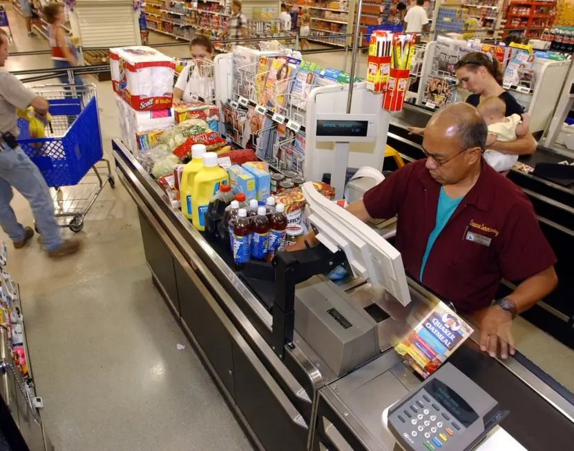
The plate shows a real warehouse and the three flows of a supply chain; the figures give the numbers of Section 3.3 and 3.4 a shape: the cost curve of the EOQ model, the stock cycle with its safety buffer and the growth of order variance up the chain.




3.6.1 Eight benefits of an ERP system for a growing company
- One version of the truth. All departments use the same database, so a sale entered once appears in stock, accounts and delivery at once. Managers no longer argue about whose spreadsheet is correct. A trading company in Birgunj can close its monthly books in days instead of weeks.
- Less duplication of work. Data is typed once and reused by every module. Clerks stop copying the same order into three registers. The time saved goes to checking and serving customers.
- Better inventory control. The system shows stock by item and by warehouse in real time and warns when the reorder point is reached. Using EOQ and safety stock, it reduces both stock-outs and idle money. A hardware wholesaler can free cash that was tied up in slow-moving goods.
- Faster, more accurate reporting. Reports of sales, profit and payables come straight from the database. Tax and audit reports are easier because the records are complete. Owners see problems while there is still time to act.
- Improved customer service. A salesperson can see stock, credit limit and delivery dates while talking to the customer. Orders are confirmed with correct dates. Customers return to suppliers that keep their promises.
- Standard processes and control. The system forces a standard way of approving purchases and payments, with a record of who approved what. This lowers the chance of fraud and mistakes. A bank or a school with many branches can apply the same rules everywhere.
- Scalability. New branches, products or users are added to the same system. A company that grows from one shop to ten does not need to start again. The cost per transaction usually falls as volume grows.
- Better planning. Linked sales, stock and production data allow forecasts and purchase plans to be made from facts. A manufacturer can plan raw materials for the festival season months ahead. Planning on facts reduces waste and rush costs.
Chapter summary
- ERP shares one database across finance, sales, procurement, inventory, manufacturing and HR; implementation may be big bang, phased, parallel or pilot, and weighted scoring supports vendor choice.
- CRM has operational, analytical and collaborative forms; RFM segments customers.
- SCM coordinates material, information and money flows. EOQ = √(2DS/H); safety stock = z·σ_d·√L; reorder point = demand × L + safety stock.
- The bullwhip effect amplifies variance up the chain by 1 + 2L/p + 2L²/p² per stage; sharing demand data and shortening lead times reduce it.
Practice
- List five ERP modules and the benefit of a single database.
- Compare big-bang and phased implementation.
- Name three types of CRM and one function of each.
- Compute the EOQ for D = 4,800 units, S = Rs 300, H = Rs 12.
- Compute safety stock for σ_d = 25, L = 4 days, 99% service (z = 2.326).
- List four causes of the bullwhip effect and two remedies.
- In the vendor scoring table, change the weights to cost 0.35 and functional fit 0.20 and recompute the winner.
- Why does 1 + 2L/p + 2L²/p² decrease when p is increased?
- How many point-to-point interfaces connect 8 systems fully, and how many connections does a bus need?
- Distinguish push from pull supply chains.
Answers and worked solutions
1. Finance, sales, procurement, inventory, manufacturing (also HR, CRM). One database means one version of the truth and no re-keying.
2. Big bang: one switch-over date, fast but risky. Phased: module by module, lower risk but needs temporary interfaces.
3. Operational (campaign and ticket automation), analytical (churn prediction), collaborative (shared customer view across channels).
4. √(2 × 4,800 × 300 / 12) = √240,000 = 489.9 units.
5. 2.326 × 25 × √4 = 116.3 units.
6. Forecast updating, order batching, price fluctuation, shortage gaming (and long lead times). Remedies: share point-of-sale data, vendor-managed inventory, smaller batches, everyday low prices.
7. New scores: X = 0.20×8 + 0.35×5 + 0.20×9 + 0.15×6 + 0.10×7 = 1.60 + 1.75 + 1.80 + 0.90 + 0.70 = 6.75. Y = 1.80 + 1.40 + 1.20 + 1.35 + 0.90 = 6.65. Z = 1.20 + 3.15 + 1.40 + 0.75 + 0.60 = 7.10. Vendor Z now wins; the ranking is sensitive to the cost weight.
8. A longer moving average reacts less to the latest demand, so the order-up-to level moves less (the terms 2L/p and 2L²/p² shrink).
9. 8 × 7 / 2 = 28 interfaces; a bus needs 8 connections.
10. Push produces from forecasts; pull produces in response to actual orders.
Model answers: medium (5 marks) and long (10 marks) questions
Q1 (5 marks). A shop sells 12,000 units a year. Ordering costs Rs 500 per order and holding costs Rs 20 per unit per year. Calculate the EOQ, number of orders, cycle time and total cost, and compare with an order size of 1,000.
Introduction. The economic order quantity is the order size that minimises the sum of annual ordering and holding costs (section 3.3, Figure 3.2).
- Formula. EOQ = square root of (2DS / H) = square root of (2 x 12,000 x 500 / 20) = square root of 600,000 = 774.6 units.
- Orders per year. 12,000 / 774.6 = 15.49 orders.
- Cycle time. 365 / 15.49 = 23.6 days between orders.
- Costs at EOQ. Ordering = 15.49 x 500 = Rs 7,746; holding = (774.6 / 2) x 20 = Rs 7,746; total = Rs 15,492. At the optimum the two are equal.
- Comparison. At Q = 1,000: ordering 12 x 500 = 6,000 and holding 500 x 20 = 10,000, total Rs 16,000, which is Rs 508 a year more.
- Assumptions. Constant demand, fixed costs, instant delivery and no discounts.
| Q | Orders | Ordering | Holding | Total (Rs) |
|---|---|---|---|---|
| 500 | 24 | 12,000 | 5,000 | 17,000 |
| 774.6 | 15.49 | 7,746 | 7,746 | 15,492 |
| 1,000 | 12 | 6,000 | 10,000 | 16,000 |
Conclusion. The EOQ balances many small orders against large stocks; because the curve is flat near the minimum, a rounded quantity close to 775 is acceptable.
Q2 (5 marks). What is the bullwhip effect? Explain its causes and the ways to reduce it, using the retailer-to-factory example.
Introduction. The bullwhip effect is the growth of the variability of orders as they move upstream from the customer to the factory (section 3.4, Figure 3.4).
- The pattern. Order variance relative to demand variance is 1.62 at the retailer, 4.06 at the wholesaler, 10.16 at the distributor and 36.82 at the factory; the standard deviation is 6.07 times larger at the factory.
- Demand forecast updating. Each stage treats the order of the next as demand and adds safety stock, so small changes are amplified.
- Order batching. Placing weekly or monthly bulk orders makes demand look lumpy.
- Price fluctuations. Discounts and promotions encourage forward buying, which then disappears.
- Rationing and gaming. When supply is short, buyers order more than they need, and then cancel.
- Remedies. Share point-of-sale data with every stage, use smaller and more frequent orders, keep stable prices, shorten lead times and use vendor-managed inventory.
Conclusion. Bullwhip is caused by the information structure of the chain, not by customers; sharing real demand data is the most effective cure.
Q3 (10 marks). Explain ERP, CRM and SCM. Show how they are integrated in an enterprise, and describe the benefits and the risks of ERP implementation.
Introduction. Large organisations need their departments to work from the same facts.
Enterprise systems provide this: ERP integrates internal processes, SCM coordinates the flow of goods with suppliers and distributors, and CRM manages relations with customers.
Together they form the backbone of the digital firm (sections 3.1 to 3.5, Figures 3.1 and 3.4).
- ERP. A suite of modules (finance, HR, sales, inventory, production, purchasing) on one shared database, so data is entered once and used everywhere.
- CRM. Stores customer contacts, orders, complaints and campaigns, and gives a complete view of each customer for sales, marketing and service.
- SCM. Plans and controls material, information and money flows from suppliers to customers: forecasting, purchasing, EOQ and safety stock, warehousing and delivery.
- Integration. A CRM order feeds ERP stock and finance, which triggers SCM replenishment and delivery; payment flows back to finance.
- Benefits. One version of the truth, less duplication, better inventory, faster reports, better service and control.
- Implementation strategies. Big bang (everything at once, fast, risky), phased (module by module, safer) and parallel (old and new together, costly).
- Risks. High cost, resistance to change, poor data migration, over-customisation and weak top-management support.
- Choosing a vendor. Use weighted scoring of fit, cost, support, scalability and local presence.
| System | Focus | Main users |
|---|---|---|
| ERP | Internal processes | All departments |
| CRM | Customers | Sales, marketing, service |
| SCM | Suppliers and delivery | Purchasing, logistics |
Conclusion. ERP, CRM and SCM share data and cover the whole business from supplier to customer. Success depends less on software than on process change, good data and committed management.