Algorithms

This closing unit steps back from individual data structures to the styles of algorithm: deterministic and non-deterministic, divide and conquer, serial and parallel, and heuristic and approximate. Knowing the styles helps you pick a strategy for a new problem.

11.1 Deterministic and non-deterministic algorithms

A deterministic algorithm has one defined next step at every point; the same input always follows the same path and gives the same output. All the algorithms in this book so far are deterministic.

A non-deterministic algorithm is a theoretical model in which a special choice step can "guess" the right option among several, and the algorithm succeeds if some sequence of guesses reaches a solution.

No real computer does this; it is a tool for classifying problems. The practical reading: a non-deterministic algorithm guesses a certificate and then verifies it with an ordinary deterministic procedure.

Class	Meaning	Examples
P	solvable in polynomial time by a deterministic algorithm	sorting, shortest path, MST
NP	a proposed solution can be verified in polynomial time (equivalently, solvable in polynomial time non-deterministically)	subset sum, Hamiltonian cycle, SAT
NP-complete	the hardest problems in NP: if one is in P, all NP is in P	SAT, travelling salesman (decision), vertex cover, knapsack (decision)

P ⊆ NP; whether P = NP is the best-known open question in computer science. For NP-complete problems no polynomial algorithm is known, so in practice we use exponential search for small inputs, or heuristic and approximate algorithms (11.5).

11.2 Divide and conquer

Divide and conquer solves a problem in three steps: divide it into smaller subproblems of the same kind, conquer them recursively (solving the smallest directly), and combine the answers. Its cost follows a recurrence T(n) = a·T(n/b) + f(n).

Master theorem (for f(n) = Θ(n^{d})): if a < b^{d} then T(n) = Θ(n^{d}); if a = b^{d} then Θ(n^{d} \log n); if a > b^{d} then Θ(n^{log_b a}).

Algorithm	Recurrence	Result
Binary search	T(n) = T(n/2) + 1	O(\log n)
Merge sort	T(n) = 2T(n/2) + n	O(n \log n)
Quick sort (balanced)	T(n) = 2T(n/2) + n	O(n \log n)
Max and min together	T(n) = 2T(n/2) + 2	3n/2 − 2 comparisons
Strassen matrix multiply	T(n) = 7T(n/2) + n²	O(n^{2}.81)
Naive recursive Fibonacci	T(n) = T(n−1) + T(n−2)	exponential: not a true divide and conquer, subproblems overlap

When subproblems overlap, divide and conquer repeats work; dynamic programming stores the answers instead.

11.3 Series (serial) and parallel algorithms

A serial algorithm executes one step at a time on one processor. A parallel algorithm splits the work among p processors that execute at the same time. Measures: speed-up S = T₁ / T_p (best serial time over parallel time) and efficiency E = S / p.

Amdahl's law. If a fraction f of the work must stay serial, the speed-up on p processors is at most S = 1 / (f + (1 − f)/p) and never exceeds 1/f however many processors are used.

Parallel problems are limited by dependencies (a step needing a previous result), communication and synchronisation costs. Merge sort, matrix multiplication, BFS levels and Monte-Carlo simulations parallelise well; computing a chain of dependent values does not.

11.4 Heuristic algorithms

A heuristic is a rule of thumb that finds a good solution quickly with no guarantee of optimality (or sometimes of success). Used when exact methods are too slow: route planning, scheduling, game playing, constraint solving.

Examples: nearest-neighbour for travelling salesman, greedy colouring, hill climbing, best-first search with an estimate function (A*, which is optimal when its estimate never overestimates).

Greedy can fail. Coins {1, 3, 4}, make 6: greedy takes 4 + 1 + 1 = 3 coins; the optimum is 3 + 3 = 2 coins.

11.5 Approximate algorithms

An approximation algorithm runs in polynomial time on an NP-hard optimisation problem and guarantees that its answer is within a known factor of optimal (the approximation ratio).

• Vertex cover, 2-approximation: repeatedly pick any uncovered edge (u, v), put both u and v in the cover, delete all edges touching them. The picked edges share no vertex, and any cover must contain at least one endpoint of each, so |optimal| ≥ number of picked edges and our cover ≤ 2 × optimal.
• Metric TSP, 2-approximation: build an MST, walk it twice (a closed tour of weight 2·MST ≤ 2·OPT), skip repeated cities by triangle inequality.

Heuristic vs approximate: both trade optimality for speed; only an approximation algorithm proves how far it can be from the best.

#include <stdio.h>
#include <string.h>

/* 1. divide and conquer: max and min together */
int cmpc;
void maxmin(const int a[], int lo, int hi, int *mx, int *mn) {
    if (lo == hi) { *mx = *mn = a[lo]; return; }
    if (hi == lo + 1) { cmpc++; if (a[lo] > a[hi]) { *mx = a[lo]; *mn = a[hi]; } else { *mx = a[hi]; *mn = a[lo]; } return; }
    int mid = (lo + hi) / 2, mx1, mn1, mx2, mn2;
    maxmin(a, lo, mid, &mx1, &mn1); maxmin(a, mid + 1, hi, &mx2, &mn2);
    cmpc += 2; *mx = mx1 > mx2 ? mx1 : mx2; *mn = mn1 < mn2 ? mn1 : mn2;
}

/* 2. non-deterministic style: verify a certificate vs brute force */
int verify(const int s[], int n, unsigned mask, int target) {
    int sum = 0; for (int i = 0; i < n; i++) if (mask >> i & 1) sum += s[i];
    return sum == target;
}

/* 3. greedy vs optimal coin change */
int greedy_coins(int amt) { int c[] = {4, 3, 1}, n = 0; for (int i = 0; i < 3; i++) { n += amt / c[i]; amt %= c[i]; } return n; }
int dp_coins(int amt)     { int dp[100] = {0}, c[] = {1, 3, 4};
    for (int a = 1; a <= amt; a++) { dp[a] = 1000; for (int i = 0; i < 3; i++) if (a >= c[i] && dp[a - c[i]] + 1 < dp[a]) dp[a] = dp[a - c[i]] + 1; }
    return dp[amt]; }

/* 4. 2-approximate vertex cover; 5. nearest-neighbour vs optimal tour */
#define V 6
#define C 5
int D[C][C] = {{0,2,9,10,7},{2,0,6,4,3},{9,6,0,8,5},{10,4,8,0,6},{7,3,5,6,0}};
int best = 1 << 30, perm[C];
void permute(int k, int len) {                       /* brute-force over tours starting at city 0 */
    if (k == C) { len += D[perm[C-1]][0]; if (len < best) best = len; return; }
    for (int i = k; i < C; i++) {
        int t = perm[k]; perm[k] = perm[i]; perm[i] = t;
        permute(k + 1, len + D[perm[k-1]][perm[k]]);
        t = perm[k]; perm[k] = perm[i]; perm[i] = t;
    }
}

int main(void) {
    int a[] = {23, 7, 91, 15, 62, 4, 38, 55};
    int mx, mn; maxmin(a, 0, 7, &mx, &mn);
    printf("max = %d, min = %d, comparisons = %d (naive would use 14)\n", mx, mn, cmpc);

    int s[] = {3, 34, 4, 12, 5, 2};
    printf("certificate {4,5} valid for 9? %s\n", verify(s, 6, (1u << 2) | (1u << 4), 9) ? "yes" : "no");
    int found = 0; unsigned tried = 0;
    for (unsigned m = 0; m < (1u << 6) && !found; m++) { tried++; found = verify(s, 6, m, 9); }
    printf("brute force tried %u of 64 subsets before success\n", tried);

    printf("make 6 from {1,3,4}: greedy %d coins, optimal %d coins\n", greedy_coins(6), dp_coins(6));

    int E[][2] = {{0,1},{0,2},{1,3},{2,3},{3,4},{4,5}}, covered[V] = {0}, size = 0;
    for (int i = 0; i < 6; i++)
        if (!covered[E[i][0]] && !covered[E[i][1]]) { covered[E[i][0]] = covered[E[i][1]] = 1; size += 2; }
    printf("2-approx vertex cover size = %d (optimal for this graph is 3)\n", size);

    int visited[C] = {1}, cur = 0, len = 0;
    printf("nearest neighbour tour: 0");
    for (int step = 1; step < C; step++) {
        int nxt = -1;
        for (int j = 0; j < C; j++) if (!visited[j] && (nxt < 0 || D[cur][j] < D[cur][nxt])) nxt = j;
        visited[nxt] = 1; len += D[cur][nxt]; cur = nxt; printf(" -> %d", cur);
    }
    len += D[cur][0]; printf(" -> 0, length %d\n", len);
    for (int i = 0; i < C; i++) perm[i] = i;
    permute(1, 0);
    printf("optimal tour length (brute force over %d tours) = %d\n", 24, best);
    return 0;
}

max = 91, min = 4, comparisons = 10 (naive would use 14)
certificate {4,5} valid for 9? yes
brute force tried 21 of 64 subsets before success
make 6 from {1,3,4}: greedy 3 coins, optimal 2 coins
2-approx vertex cover size = 6 (optimal for this graph is 3)
nearest neighbour tour: 0 -> 1 -> 4 -> 2 -> 3 -> 0, length 28
optimal tour length (brute force over 24 tours) = 26

11.6 Seeing the ideas: many ways to design an algorithm

Different problems need different design strategies. Some problems split neatly into halves (divide and conquer). Some can be shared among many processors at once.

Some are so hard that an exact answer is out of reach and a good answer found quickly has to do (heuristic and approximate methods).

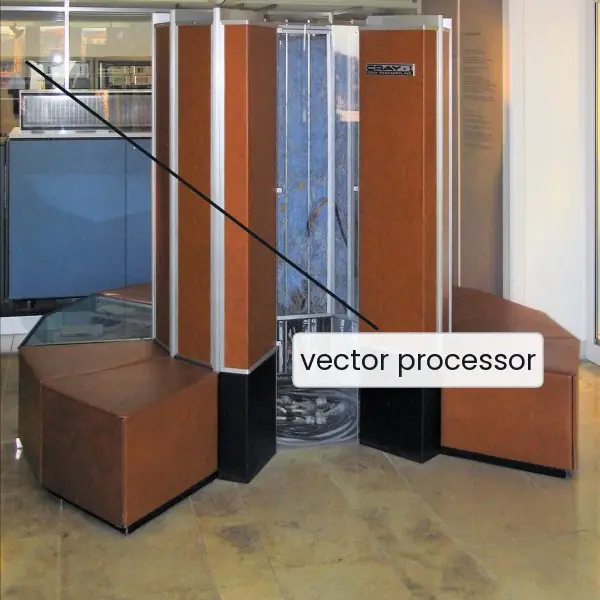
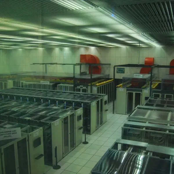
The photographs show the machines on which the parallel idea grew: the Cray-1 of 1976, the first commercial vector supercomputer; a modern graphics card whose thousands of small cores work on one problem together; and the computer centre at CERN where thousands of machines share one analysis.

(a) Cray-1 supercomputer (1976)

(b) Graphics card: many cores, one job

(c) CERN computer centre (parallel farm)

11.6.1 Eight points on choosing and using algorithm design methods

1. Divide and conquer breaks big problems into small ones. Merge sort, quick sort and binary search split the problem, solve the parts and combine the answers. The recurrence T(n) = 2T(n/2) + n gives O(n \log n), as in Figure 11.1. It is the method to try first when a problem has the same form at every size.
2. Parallel algorithms use many processors together. The sum of 8 numbers needs only 3 parallel steps instead of 7 (Figure 11.2). Weather forecasting, image processing and the training of machine-learning models run on graphics cards for this reason. Nepal's weather and flood forecasts at the Department of Hydrology and Meteorology rely on such computing.
3. Amdahl's law limits parallel speed-up. The sequential part of a program always remains, so extra processors help less and less. With 90 per cent parallel work the speed-up can never pass 10, even with 1,000 processors. Programmers therefore first reduce the sequential part.
4. Deterministic algorithms are predictable. For the same input they follow the same steps and give the same output. All the programs in this book are deterministic. This makes them easy to test and to prove correct.
5. Non-deterministic algorithms describe hard problems. They are imagined to guess the right choice and then verify it, as in Figure 11.4. They do not run on real computers but they define the class NP. Many practical problems, such as timetabling and route planning with many stops, belong to this class.
6. Heuristics give good answers fast. A heuristic is a rule of thumb that is not guaranteed to find the best answer. The nearest-neighbour rule found a tour of length 38 against the optimum 32, but needed very few steps (Figure 11.3). A delivery company in Kathmandu uses such rules daily because exact search would take far too long.
7. Approximation algorithms give guarantees. Unlike a plain heuristic, an approximation algorithm proves that its answer is within a known factor of the optimum. The vertex-cover method is never worse than twice the best. This is useful when a wrong answer would be costly and the optimum is out of reach.
8. The choice depends on size and cost of error. For small inputs an exact search is best, for large inputs with a time limit a heuristic or approximation is used, and for huge inputs parallel processing helps. A good programmer states which method was used and how far from the best the answer may be. Knowing the options is part of professional practice.

(a) A postman's bicycle: a round of many stops

(b) Nearest neighbour vs exact shortest round

Formula and fact sheet

• P ⊆ NP; NP-complete = hardest in NP; verifying a certificate is polynomial.
• Master theorem: T(n) = aT(n/b) + Θ(n^{d}): a < b^{d} → n^{d}; a = b^{d} → n^{d} log n; a > b^{d} → n^{log_b a}.
• Speed-up S = T₁/T_p; Amdahl: S ≤ 1/(f + (1−f)/p) ≤ 1/f.
• Heuristic: no guarantee. Approximation: guaranteed ratio (vertex cover 2).
• Greedy optimal for Huffman, MST, Dijkstra; not for arbitrary coin systems.

Chapter summary

• Deterministic algorithms follow one path; non-deterministic ones guess and verify, which defines NP.
• Divide and conquer splits, solves and combines; recurrences and the Master theorem give the cost.
• Parallel algorithms speed up only the parallelisable fraction (Amdahl's law).
• For hard problems we accept heuristics (no guarantee) or approximation algorithms (guaranteed ratio).

Practice

1. Differentiate deterministic and non-deterministic algorithms.
2. Define P, NP and NP-complete; give an example of each.
3. Solve T(n) = 4T(n/2) + n and T(n) = 2T(n/2) + n² using the Master theorem.
4. Explain the divide, conquer and combine steps of merge sort on 6 4 9 1.
5. A program is 80% parallelisable. Find the maximum speed-up on 4 processors and with infinite processors.
6. Compare heuristic and approximate algorithms.
7. Show that greedy coin change fails for coins {1, 3, 4} and amount 6.
8. Explain why the 2-approximation for vertex cover is within a factor of 2.
9. When is divide and conquer a poor choice?

Answers and worked solutions

1. Deterministic: every step is fully determined, so one run per input. Non-deterministic: may choose among options, accepting if any choice sequence succeeds; used as a theoretical model.

2. P: solvable in polynomial time (sorting). NP: solutions verifiable in polynomial time (subset sum). NP-complete: NP problems to which every NP problem reduces (SAT, decision TSP).

3. a = 4, b = 2, d = 1: a > b^{d} (4 > 2) → Θ(n^{log₂4}) = Θ(n²). Second: a = 2, b = 2, d = 2: a < b^{d} (2 < 4) → Θ(n²).

4. Divide: [6 4] [9 1]. Conquer: sort each: [4 6] [1 9]. Combine: merge → [1 4 6 9].

5. f = 0.2. p = 4: 1/(0.2 + 0.8/4) = 1/0.4 = 2.5. p → ∞: 1/0.2 = 5.

6. Both are used for hard problems and trade exactness for speed. A heuristic gives no bound on how far it can be from the optimum; an approximation algorithm guarantees a ratio.

7. Greedy: 4 + 1 + 1 = 3 coins. Optimal: 3 + 3 = 2 coins.

8. The edges selected share no endpoint (a matching of size k). Any cover needs one endpoint per selected edge, so OPT ≥ k, while the algorithm uses 2k vertices ≤ 2·OPT.

9. When the subproblems overlap heavily (naive Fibonacci), repeating the work makes it exponential; use dynamic programming instead. It is also unhelpful when dividing and combining cost more than solving directly.

Model answers (5 and 10 marks)

Q1. Explain the divide and conquer method with an example and its general recurrence. (5 marks)

Divide and conquer solves a problem in three steps: (1) divide the problem into smaller sub-problems of the same kind, (2) conquer each sub-problem recursively (a very small problem is solved directly), and (3) combine the sub-answers into the answer to the whole problem.

Example: merge sort. Divide an array of n items into two halves; sort each half by the same method; merge the two sorted halves in O(n) time. If T(n) is the time, then T(n) = 2 T(n / 2) + n with T(1) = 1.

Solution. For n = 8 the recursion tree has 4 levels (Figure 11.1); each level does 8 units of work (the splitting and merging at that level), so the total is 8 x 4 = 32 = n (log2 n + 1), that is O(n \log n).

General form. T(n) = a T(n / b) + f(n), where a is the number of sub-problems, n / b the size of each and f(n) the cost of dividing and combining.

Other examples are binary search, T(n) = T(n / 2) + 1, which gives O(\log n), quick sort, and Strassen's matrix multiplication. The method is suitable when sub-problems are independent and of the same form.

It fits parallel computers well, because the sub-problems can be solved at the same time.

Q2. Differentiate between serial and parallel algorithms and state Amdahl's law. (5 marks)

A serial (sequential) algorithm executes one instruction at a time on one processor. A parallel algorithm splits the work into parts that run at the same time on several processors or cores, then combines the results.

Point	Serial	Parallel
Processors	one	many
Execution	one step after another	simultaneous steps
Time for adding 8 numbers	7 steps	3 steps with 4 processors
Difficulty	simple to design and debug	needs splitting, synchronisation, communication
Hardware	any computer	multi-core CPU, GPU, cluster
Examples	linear search, simple loops	matrix multiplication, image filters, weather models

Amdahl's law. If a fraction p of a program can be parallelised and N processors are used, the speed-up is S = 1 / ((1 - p) + p / N). For p = 0.9: S = 1.82 for N = 2, 3.08 for N = 4, 6.40 for N = 16 and 9.91 for N = 1,000.

The speed-up can never exceed 1 / (1 - p) = 10, because the sequential tenth cannot be shortened (Figure 11.2).

The law tells us that reducing the sequential part is more valuable than adding processors, and that parallel algorithms need extra care for communication and synchronisation.

Q3. Explain heuristic and approximate algorithms with examples, and compare them with exact algorithms. Illustrate with the travelling salesman and vertex cover problems. (10 marks)

Introduction. Some problems, such as the travelling salesman problem (TSP) and vertex cover, are NP-hard: no known algorithm solves every instance quickly.

For 20 towns, an exact search must check (20 - 1)! / 2 = 60,822,550,204,416,000 tours, which is impossible. In practice we accept a good answer found fast, using heuristic or approximation methods.

Heuristic algorithm. A heuristic is a rule of thumb that usually gives a good answer quickly but has no guarantee of optimality.

Example: nearest-neighbour TSP Start at a town and always move to the nearest unvisited town. For the five towns of Figure 11.3 starting at A, the tour is A, E, B, C, D, A with length 8 + 2 + 3 + 6 + 19 = 38.

The exact method, which checks all 12 distinct tours, finds A, C, B, D, E, A with length 10 + 3 + 7 + 4 + 8 = 32. The heuristic is 18.75 per cent longer, but its time is only O(n squared).

Other heuristics are hill climbing, greedy choices, and rules used in game playing.

Approximation algorithm. An approximation algorithm runs in polynomial time and guarantees that its answer is within a known factor of the optimum, the approximation ratio.

Example: vertex cover A vertex cover is a set of vertices that touches every edge. Repeat: pick any edge not yet covered and add both its end points to the cover.

On the path 1-2-3-4-5-6 this picks edges 1-2, 3-4 and 5-6 and gives a cover of 6 vertices, while the optimum {2, 4, 5} has 3.

The chosen edges share no end point, so any cover needs at least one vertex from each of them; the optimum is at least the number of chosen edges, and our cover has twice that number. Hence the ratio is at most 2.

Point	Exact algorithm	Heuristic	Approximation algorithm
Answer	always optimal	good, not guaranteed	within a proven factor
Time	exponential for NP-hard problems	usually short	polynomial
Proof of quality	by correctness proof	none, tested by experiment	proven ratio
Example	try all TSP tours	nearest neighbour	2-approximation vertex cover
Use	small inputs	large inputs, speed matters	large inputs, quality bound matters

Link with deterministic and non-deterministic algorithms. A deterministic algorithm follows one fixed sequence of steps.

A non-deterministic algorithm is imagined to guess correctly and then verify the guess quickly; the problems solvable this way in polynomial time form class NP.

In the subset-sum question of Figure 11.4 the guess {4, 5} is verified in a few steps, but a deterministic search may need 2 to the power n subsets (1,073,741,824 for n = 30).

Whether P equals NP is the most famous open problem of the subject.

Conclusion. Choose an exact algorithm when the input is small, a heuristic when speed matters more than perfection, and an approximation algorithm when a guaranteed bound is needed.

Divide and conquer and parallel processing can then speed up whichever method is chosen.