Unit 10 · 5 teaching hours · 24 min read
Graphs
What the syllabus asks for 8
- Graphs as an ADT; types of graph
- Representations
- Transitive closure and Warshall's algorithm
- Traversal and spanning forests
- Minimum spanning trees (Kruskal and round-robin)
- Shortest paths: the greedy method and Dijkstra
- Programs: BFS, DFS, Dijkstra, Kruskal, Warshall
- Seeing the ideas: graphs of bridges, roads and routes
A graph G = (V, E) is a set of vertices (nodes) and a set of edges joining pairs of vertices. Graphs model road maps, networks, social connections, dependencies and the web. This unit covers representations, closure, traversal, spanning trees and shortest paths.
- The graph ADT, terminology and types of graph.
- Adjacency matrix and list; transitive closure by Warshall's algorithm.
- BFS and DFS traversals, spanning forests.
- Kruskal's and round-robin minimum spanning tree algorithms, Dijkstra's shortest path, the greedy method.
10.1 Graphs as an ADT; types of graph
Operations: add/remove vertex, add/remove edge, adjacent(u, v), neighbours(v), traverse.
| Term | Meaning |
|---|---|
| Undirected / directed (digraph) | edges have no direction / edges are ordered pairs u → v |
| Weighted | each edge carries a cost or length |
| Degree | edges at a vertex (digraph: in-degree and out-degree). Σ degrees = 2 |
| Path / cycle | sequence of edges / a path that returns to its start |
| Connected | a path exists between every pair (digraph: strongly connected if in both directions) |
| Tree | connected graph with no cycles: |
| Complete graph | every pair adjacent: |
| Simple / multigraph | no loops or parallel edges / allows them |
| DAG | directed acyclic graph (task dependencies, topological order) |
| Sparse / dense |
10.2 Representations
| Adjacency matrix | Adjacency list | |
|---|---|---|
| Structure | n × n array, A[i][j] = 1 (or weight) if edge i–j | array of linked lists of neighbours |
| Space | O(n²) | O(n + e) |
| Edge test (u, v) | O(1) | O(degree) |
| List all neighbours | O(n) | O(degree) |
| Best for | dense graphs, Warshall | sparse graphs, traversal |
For an undirected graph the matrix is symmetric.
10.3 Transitive closure and Warshall's algorithm
The transitive closure of a digraph has an edge u → v whenever a path from u to v exists. It answers "is v reachable from u?" for all pairs.
Warshall's algorithm starts with the adjacency matrix R and, for each intermediate vertex k in turn, sets R[i][j] = R[i][j] OR (R[i][k] AND R[k][j]).
After processing k, R[i][j] = 1 iff there is a path from i to j using only vertices 0..k as intermediates. Time O(n³), space O(n²).
Digraph 0 → 1, 1 → 2, 2 → 3. k = 0: nothing is routed through 0 except into it (no new edges). k = 1: 0 → 1 and 1 → 2 give 0 → 2. k = 2: 0 → 2, 1 → 2 and 2 → 3 give 0 → 3 and 1 → 3. k = 3: no new edges. The closure has six edges: 0→1, 0→2, 0→3, 1→2, 1→3, 2→3.
10.4 Traversal and spanning forests
Breadth-first search (BFS): visit the start vertex, then all its neighbours, then their neighbours, level by level, using a queue. It finds the fewest-edge path in an unweighted graph.
Depth-first search (DFS): go as deep as possible along one path, then backtrack, using a stack (or recursion). It detects cycles and underlies topological sorting and connected components.
Both take O(n + e) with adjacency lists (O(n²) with a matrix).
The edges used to discover new vertices form a spanning tree of the component (the BFS tree or DFS tree). If the graph is disconnected, restarting the search from each unvisited vertex produces a spanning forest: one tree per component.
10.5 Minimum spanning trees (Kruskal and round-robin)
A spanning tree connects all n vertices with n − 1 edges and no cycle. In a weighted graph the minimum spanning tree (MST) has the least total weight (cabling a network at minimum cost).
Kruskal's algorithm. Sort the edges by weight; take each edge in turn unless it would form a cycle with edges already chosen (tested with union-find); stop at n − 1 edges. O(e \log e).
Round-robin algorithm (Sollin/Borůvka family). Keep a queue of trees, initially every vertex alone.
Repeatedly remove the tree at the front, find the cheapest edge leaving it, add that edge (merging it with another tree) and put the merged tree at the back. Stop when one tree remains.
It is correct because the cheapest edge leaving any tree always belongs to some MST (the cut property).
Prim's algorithm grows one tree from a start vertex by repeatedly adding the cheapest edge to a new vertex.
10.6 Shortest paths: the greedy method and Dijkstra
A greedy algorithm builds a solution by always taking the best-looking choice at the moment, never reconsidering.
It is correct only for problems with the greedy-choice property (Huffman, Kruskal, Prim, Dijkstra, fractional knapsack); for others it only approximates (Unit 11).
Dijkstra's algorithm finds shortest paths from one source in a graph with non-negative weights. Keep dist[v] (∞ initially, 0 for the source).
Repeat: pick the unfinished vertex u with the smallest dist; mark it final; for each neighbour v relax: if dist[u] + w(u, v) < dist[v], update dist[v] and set the predecessor. O(n²) with an array, O((n + e) log n) with a heap.
It fails with negative edges (use Bellman-Ford).
Graph (undirected, weights): 0–1: 7, 0–2: 9, 0–5: 14, 1–2: 10, 1–3: 15, 2–3: 11, 2–5: 2, 3–4: 6, 4–5: 9. Source 0. Start dist = [0, ∞, ∞, ∞, ∞, ∞]. Finalise 0: dist 1 = 7, 2 = 9, 5 = 14.
Finalise 1 (7): 3 = 22 (7 + 15); 2 stays 9 (7 + 10 = 17). Finalise 2 (9): 3 = 20, 5 = 11. Finalise 5 (11): 4 = 20. Finalise 3 (20) and 4 (20). Final distances: 1: 7, 2: 9, 3: 20, 4: 20, 5: 11. Path to 4: 0 → 2 → 5 → 4.
Kruskal on the same graph: edges by weight 2 (2–5), 6 (3–4), 7 (0–1), 9 (0–2), 9 (4–5), 10 (1–2, cycle), 11 (2–3, cycle), …. Chosen: 2–5, 3–4, 0–1, 0–2, 4–5: total 33 with 5 edges for 6 vertices.
Round robin: queue {0},{1},{2},{3},{4},{5}. {0} takes its cheapest edge 0–1 (7); the merged tree {0,1} goes to the back and {1} leaves the queue. {2} takes 2–5 (2) → {2,5}. {3} takes 3–4 (6) → {3,4}. {0,1} takes its cheapest leaving edge 0–2 (9) → {0,1,2,5}. {3,4} takes 4–5 (9) and everything is joined. Same five edges, total 33.
10.7 Programs: BFS, DFS, Dijkstra, Kruskal, Warshall
The first program builds the example graph and runs BFS, DFS and Dijkstra; the second runs Kruskal's algorithm and Warshall's closure.
#include <stdio.h>
#define N 6
#define INF 1000000
int w[N][N];                         /* weighted adjacency matrix, 0 = no edge */
void add(int u, int v, int c) { w[u][v] = w[v][u] = c; }
void graph(void) {
    add(0,1,7); add(0,2,9); add(0,5,14); add(1,2,10); add(1,3,15);
    add(2,3,11); add(2,5,2); add(3,4,6); add(4,5,9);
}

void bfs(int s) {
    int q[N], f = 0, r = 0, seen[N] = {0};
    q[r++] = s; seen[s] = 1;
    while (f < r) {
        int u = q[f++]; printf("%d ", u);
        for (int v = 0; v < N; v++) if (w[u][v] && !seen[v]) { seen[v] = 1; q[r++] = v; }
    }
}
int vis[N];
void dfs(int u) {
    vis[u] = 1; printf("%d ", u);
    for (int v = 0; v < N; v++) if (w[u][v] && !vis[v]) dfs(v);
}
void dijkstra(int s) {
    int d[N], done[N] = {0}, pred[N];
    for (int i = 0; i < N; i++) { d[i] = INF; pred[i] = -1; }
    d[s] = 0;
    for (int it = 0; it < N; it++) {
        int u = -1;
        for (int i = 0; i < N; i++) if (!done[i] && (u < 0 || d[i] < d[u])) u = i;
        done[u] = 1;
        for (int v = 0; v < N; v++)
            if (w[u][v] && d[u] + w[u][v] < d[v]) { d[v] = d[u] + w[u][v]; pred[v] = u; }
    }
    for (int i = 0; i < N; i++) {
        printf("  to %d: dist %2d, path:", i, d[i]);
        int path[N], k = 0; for (int x = i; x != -1; x = pred[x]) path[k++] = x;
        while (k--) printf(" %d", path[k]);
        printf("\n");
    }
}

int main(void) {
    graph();
    printf("BFS from 0: "); bfs(0);
    printf("\nDFS from 0: "); dfs(0);
    printf("\nDijkstra from 0:\n"); dijkstra(0);
    return 0;
}
BFS from 0: 0 1 2 5 3 4
DFS from 0: 0 1 2 3 4 5
Dijkstra from 0:
  to 0: dist  0, path: 0
  to 1: dist  7, path: 0 1
  to 2: dist  9, path: 0 2
  to 3: dist 20, path: 0 2 3
  to 4: dist 20, path: 0 2 5 4
  to 5: dist 11, path: 0 2 5
#include <stdio.h>
#define N 6
#define INF 1000000
int w[N][N];                         /* weighted adjacency matrix, 0 = no edge */
void add(int u, int v, int c) { w[u][v] = w[v][u] = c; }
void graph(void) {
    add(0,1,7); add(0,2,9); add(0,5,14); add(1,2,10); add(1,3,15);
    add(2,3,11); add(2,5,2); add(3,4,6); add(4,5,9);
}

int parent[N];
int find(int x) { return parent[x] == x ? x : (parent[x] = find(parent[x])); }

int main(void) {
    graph();
    int eu[20], ev[20], ec[20], m = 0;                 /* collect and sort the edges by weight */
    for (int i = 0; i < N; i++) for (int j = i + 1; j < N; j++) if (w[i][j]) { eu[m] = i; ev[m] = j; ec[m] = w[i][j]; m++; }
    for (int i = 0; i < m; i++) for (int j = 0; j < m - 1 - i; j++) if (ec[j] > ec[j+1]) {
        int t; t = eu[j]; eu[j] = eu[j+1]; eu[j+1] = t; t = ev[j]; ev[j] = ev[j+1]; ev[j+1] = t; t = ec[j]; ec[j] = ec[j+1]; ec[j+1] = t; }
    for (int i = 0; i < N; i++) parent[i] = i;
    int total = 0;
    printf("Kruskal MST edges:");
    for (int i = 0; i < m; i++) {
        int x = find(eu[i]), y = find(ev[i]);
        if (x != y) { parent[x] = y; total += ec[i]; printf(" (%d-%d:%d)", eu[i], ev[i], ec[i]); }
    }
    printf("\nMST total weight = %d\n", total);

    int R[4][4] = {{0,1,0,0},{0,0,1,0},{0,0,0,1},{0,0,0,0}};      /* Warshall: digraph 0->1->2->3 */
    for (int k = 0; k < 4; k++) for (int i = 0; i < 4; i++) for (int j = 0; j < 4; j++)
        R[i][j] = R[i][j] || (R[i][k] && R[k][j]);
    printf("Warshall closure:\n");
    for (int i = 0; i < 4; i++) { printf("  "); for (int j = 0; j < 4; j++) printf("%d ", R[i][j]); printf("\n"); }
    return 0;
}
Kruskal MST edges: (2-5:2) (3-4:6) (0-1:7) (0-2:9) (4-5:9)
MST total weight = 33
Warshall closure:
  0 1 1 1
  0 0 1 1
  0 0 0 1
  0 0 0 0
10.8 Seeing the ideas: graphs of bridges, roads and routes
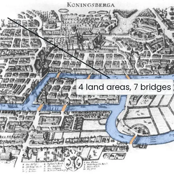
Graph theory began with a walk. In 1736 the people of Königsberg (now Kaliningrad) wondered whether one could cross each of the city's seven bridges exactly once and return home.
Leonhard Euler proved that it was impossible by replacing the map with a graph of four land masses and seven bridges.
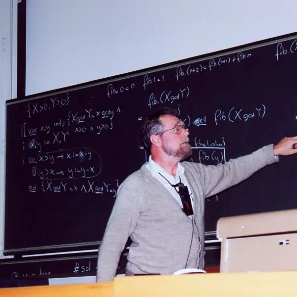
In 1956 Edsger Dijkstra designed his shortest-path algorithm in about twenty minutes, without pencil and paper, to show off a computer's ability to find a route between two Dutch cities.
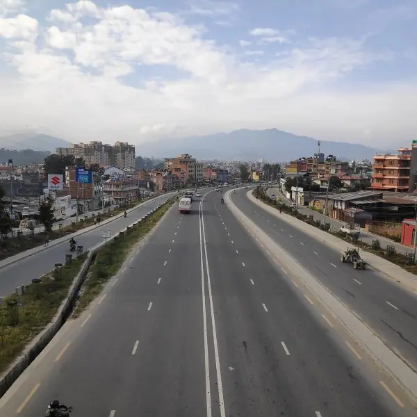
Today the same idea finds the best route on the Kathmandu Ring Road.


10.8.1 Eight applications of graphs
- Maps and route finding. Road maps are weighted graphs whose vertices are junctions and whose edges are road sections. Ride-hailing and map applications run Dijkstra-type algorithms to find the quickest route through the Kathmandu valley. The edge weight can be distance, time or toll cost.
- Computer networks. The internet is a graph of routers joined by links. Routing protocols such as OSPF use shortest-path algorithms to choose where to send each packet. When a link fails, the graph is updated and new routes are found.
- Social networks. People are vertices and friendships are edges. Platforms use traversals to suggest friends of friends and to measure how closely two people are connected. Telecom companies such as Nepal Telecom study call graphs in the same way.
- Telecommunication and utility design. A minimum spanning tree gives the cheapest way to connect all towns, villages or buildings with cable, pipe or fibre. For the graph of Figure 10.3 the cheapest network costs 13 units. Planners of hydropower transmission lines and rural internet networks use it.
- Project scheduling. Tasks and their dependencies form a directed graph, and a topological order gives a valid sequence. The longest path through it is the critical path that decides the project time. A construction plan for a bridge or a software project uses this.
- Web crawling and search engines. Web pages are vertices and hyperlinks are edges. A crawler visits pages by BFS, and ranking methods study the link structure. Every search result you see began with a graph traversal.
- Dependency and prerequisite checking. Course prerequisites at a university, package dependencies in software and build orders in a compiler form directed graphs. A cycle in the graph means an impossible requirement. DFS detects such a cycle.
- Puzzles and artificial intelligence. Each state of a puzzle is a vertex and each legal move is an edge. BFS finds the shortest solution of a sliding puzzle, and game-playing programs search graphs of positions. The Königsberg problem itself, with its odd degrees, is the first example.



Formula and fact sheet
- Σ deg(v) = 2|E|. Complete graph: n(n−1)/2 edges. Tree: n − 1 edges.
- Matrix O(n²) space; list O(n + e). BFS/DFS O(n + e) with lists.
- BFS = queue, shortest in edges; DFS = stack/recursion.
- Warshall: R[i][j] |= R[i][k] & R[k][j]; O(n³).
- MST: Kruskal O(e \log e); cut property justifies Kruskal, Prim and round robin.
- Dijkstra: non-negative weights; relax dist[v] = min(dist[v], dist[u] + w).
Chapter summary
- Graphs generalise trees; representation decides the cost of each operation.
- Warshall's algorithm computes reachability; BFS and DFS traverse in O(n + e) and produce spanning trees or forests.
- Kruskal and round-robin build minimum spanning trees greedily; Dijkstra computes shortest paths greedily.
- Greedy works only when the greedy-choice property holds.
Practice
- Define graph, degree, path, cycle, connected graph, tree.
- A graph has degrees 3, 3, 2, 2, 2. How many edges? Draw an adjacency matrix for the triangle 1–2–3.
- Compare adjacency matrix and list for a graph with 1,000 vertices and 3,000 edges.
- Perform BFS and DFS from A on edges A–B, A–C, B–D, C–D, D–E (neighbours in alphabetical order).
- Apply Warshall's algorithm to the digraph 0→1, 1→2, 2→0, 2→3.
- Find the MST of: A–B 4, A–C 1, B–C 2, B–D 5, C–D 8, C–E 10, D–E 2 using Kruskal.
- Run Dijkstra from A on A–B 4, A–C 2, B–C 1, B–D 5, C–D 8, D–E 3.
- Why does Dijkstra fail with negative edges? Give an example.
- State the cut property and say how it justifies Kruskal's algorithm.
Answers and worked solutions
1. Graph: vertices plus edges. Degree: edges at a vertex. Path: sequence of adjacent edges. Cycle: path returning to its start. Connected: a path between every pair. Tree: connected and acyclic.
2. Σ degrees = 12, so |E| = 6. Triangle matrix rows: 1: 0 1 1; 2: 1 0 1; 3: 1 1 0.
3. Matrix: 10⁶ cells. List: about 1,000 + 2·3,000 = 7,000 entries. The list is far smaller; the matrix tests a single edge in O(1).
4. BFS: A, B, C, D, E. DFS: A, B, D, C, E (A → B → D → then C via D, back, then E from D: visiting order A B D C E).
5. Edges 0→1, 1→2, 2→0, 2→3. Following paths: 0 reaches 1, 2, 0 (around the cycle) and 3; 1 reaches 2, 0, 1 and 3; 2 reaches 0, 1, 2 and 3; 3 reaches nothing. So the closure matrix has every entry 1 in rows 0–2 and a zero row for vertex 3. (Warshall reaches this by adding 2→1 at k = 0, then 0→2, 2→2 at k = 1, and the remaining pairs at k = 2.)
6. Edges by weight: A–C 1, B–C 2, D–E 2, B–D 5 (A–B 4 would form a cycle A–C–B, skip), then B–D joins {A,B,C} with {D,E}. Chosen: A–C, B–C, D–E, B–D: total 1 + 2 + 2 + 5 = 10.
7. A 0; C 2 (A–C); B 3 (via C: 2 + 1); D 8 (via B: 3 + 5; via C: 2 + 8 = 10); E 11 (8 + 3). Paths: A–C–B–D–E.
8. Dijkstra finalises a vertex when it is the closest unfinished one, assuming later paths can only be longer; a negative edge can make a later path shorter. Example: A→B 2, A→C 3, C→B −2: Dijkstra finalises B at 2 but the true shortest A→B is 1.
9. For any cut of the vertices, the lightest edge crossing it belongs to some MST. Kruskal's next edge is the lightest edge between two different components, i.e. across a cut separating them, so it is always safe.
Model answers (5 and 10 marks)
Q1. Define a graph and explain its terms and representations. (5 marks)
A graph G = (V, E) consists of a set V of vertices (nodes) and a set E of edges that connect pairs of vertices.
In an undirected graph an edge has no direction; in a directed graph (digraph) each edge goes from one vertex to another; in a weighted graph each edge has a number such as distance or cost (Plate 10.1c).
Terms. Two vertices are adjacent if an edge joins them. The degree of a vertex is the number of edges at it (in a digraph, in-degree and out-degree).
A path is a sequence of vertices joined by edges, a cycle is a path that returns to its start, and a graph is connected if every vertex can be reached from every other.
A tree is a connected graph with no cycle, and a graph with V vertices has at most V(V - 1)/2 edges if undirected.
Representations. For the graph with vertices A, B, C, D and edges A-B, A-C, B-C, C-D:
| A | B | C | D | |
|---|---|---|---|---|
| A | 0 | 1 | 1 | 0 |
| B | 1 | 0 | 1 | 0 |
| C | 1 | 1 | 0 | 1 |
| D | 0 | 0 | 1 | 0 |
- Adjacency matrix: a V x V array, as above. It uses O(V squared) space, tests an edge in O(1), and is good for dense graphs.
- Adjacency list: A: B, C; B: A, C; C: A, B, D; D: C. It uses O(V + E) space (here 4 + 8 = 12 entries) and is good for sparse graphs such as road maps.
Q2. Compare breadth-first search and depth-first search. (5 marks)
Both algorithms visit every vertex reachable from a start vertex exactly once and mark visited vertices so that cycles do not cause endless loops. With adjacency lists both take O(V + E) time.
BFS visits the start vertex, then all its neighbours, then their neighbours, level by level. It uses a queue: dequeue a vertex, enqueue its unvisited neighbours. DFS goes as deep as possible along one path and then backtracks.
It uses a stack or recursion: push a vertex, move to an unvisited neighbour, pop when none is left.
For the graph of Figure 10.2 from A with neighbours in alphabetical order, BFS gives A B C D E F and DFS gives A B D C E F.
| Point | BFS | DFS |
|---|---|---|
| Data structure | queue | stack / recursion |
| Order | level by level | deep first |
| Shortest path (unweighted) | yes | not guaranteed |
| Memory | can be large (whole level) | proportional to depth |
| Typical uses | shortest path, web crawling, friend suggestion | cycle detection, topological sort, maze solving |
BFS is chosen when the nearest answer is needed; DFS is chosen to explore all possibilities, detect cycles and order tasks.
Q3. Explain Dijkstra's shortest-path algorithm and apply it to the graph with edges A-B 4, A-C 2, B-C 1, B-D 5, C-D 8, C-E 10, D-E 2, D-F 6, E-F 3 from source A. (10 marks)
Introduction. Dijkstra's algorithm (1956, published 1959) finds the shortest path from one source vertex to every other vertex in a graph with non-negative edge weights.
It is a greedy algorithm: it always fixes the nearest unfixed vertex next, and that distance can never be improved later.
Algorithm.
- Set
dist[source] = 0anddist[v] = infinityfor every other vertex; mark all vertices unvisited; setprev[v]to none. - Choose the unvisited vertex
uwith the smallestdist[u]and mark it visited (its distance is final). - For every unvisited neighbour
vofu: ifdist[u] + w(u, v) < dist[v], setdist[v] = dist[u] + w(u, v)andprev[v] = u. This step is called relaxation. - Repeat steps 2 and 3 until all vertices are visited or the smallest distance is infinity.
- Read a path backwards from the target through
prev.
Worked example (Figure 10.3).
| Step | Vertex fixed | A | B | C | D | E | F |
|---|---|---|---|---|---|---|---|
| Start | 0 | inf | inf | inf | inf | inf | |
| 1 | A (0) | 0 | 4 | 2 | inf | inf | inf |
| 2 | C (2) | 0 | 3 | 2 | 10 | 12 | inf |
| 3 | B (3) | 0 | 3 | 2 | 8 | 12 | inf |
| 4 | D (8) | 0 | 3 | 2 | 8 | 10 | 14 |
| 5 | E (10) | 0 | 3 | 2 | 8 | 10 | 13 |
| 6 | F (13) | 0 | 3 | 2 | 8 | 10 | 13 |
The shortest distances from A are B 3, C 2, D 8, E 10 and F 13. The path to F is read backwards: F came from E, E from D, D from B, B from C, C from A, so the route is A - C - B - D - E - F with length 2 + 1 + 5 + 2 + 3 = 13.
Complexity. With an adjacency matrix or a simple array search for the minimum the time is O(V squared); with adjacency lists and a binary heap (priority queue) it is O((V + E) log V). Space is O(V).
The method fails if an edge weight is negative, for which Bellman-Ford is used instead. A BFS gives the same answer only when all weights are equal.
Conclusion. Dijkstra's algorithm is the basis of route finding in maps and routing protocols. Its correctness rests on the greedy choice of the nearest unfixed vertex and on non-negative weights.