Unit 1 · 2 teaching hours · 16 min read
Introduction to Data Structure
What the syllabus asks for 6
- Data, data structure and algorithm
- Abstract Data Type
- Why data structures matter
- Measuring cost in one page
- Conventions in this book
- Seeing the ideas: algorithms, structures and cost
Every program stores data and does something with it. A data structure is a disciplined way of organising data so that the operations you need are fast and simple; an algorithm is the step-by-step procedure that uses it.
Choosing the right structure is usually the difference between a program that answers instantly and one that never finishes.
- A precise definition of data structure and the standard classification.
- The idea of an Abstract Data Type (ADT): what a structure does, separated from how.
- A first look at measuring cost, which Unit 8 develops fully.
- A guide for choosing a structure, and the C conventions used in the rest of the book.
1.1 Data, data structure and algorithm
Data are raw values (a roll number, a name, a mark). A data structure is a collection of data values, the relationships among them, and the operations that can be applied to them.
An array of marks, a list of students and a tree of folders are data structures. An algorithm is a finite sequence of unambiguous steps that takes input and produces output, and always stops.
Niklaus Wirth's slogan sums up the subject: Algorithms + Data Structures = Programs.
Classification
| Basis | Classes | Examples |
|---|---|---|
| Primitive or not | Primitive (built into the language) · Non-primitive (built from primitives) | int, char, float · array, struct, list, tree |
| Shape | Linear (elements in a sequence, one predecessor and one successor) · Non-linear (one element may link to many) | array, stack, queue, linked list · tree, graph |
| Size | Static (fixed size at compile time) · Dynamic (grows and shrinks at run time) | array · linked list |
| Order of access | Sequential · Random | tape, linked list · array |
Non-primitive linear structures covered in this book: arrays, stack, queue, list and linked list (Units 2–5). Non-linear: trees and graphs (Units 7 and 10).
1.2 Abstract Data Type
An Abstract Data Type (ADT) is a mathematical model of a data structure defined by what it stores and what operations it supports, with no mention of how it is coded. The user sees only the interface; the implementer is free to change the inside.
Data: a collection of items in which only the most recently added one is accessible. Operations: push(x) add item · pop() remove and return the top · peek() read the top · isEmpty() · isFull().
Rules: pop on an empty stack is an underflow error; push on a full one is an overflow. The same ADT can be implemented with an array (Unit 2) or a linked list (Unit 5).
A program that only calls push and pop does not change when the implementation does. That independence is the whole point of an ADT.
In C an ADT becomes a struct plus a set of functions that take a pointer to it:
typedef struct { int items[100]; int top; } Stack;   /* the representation */
void stack_init(Stack *s);                           /* the interface      */
void push(Stack *s, int x);
int  pop(Stack *s);
Three levels of thought: the logical level (the ADT), the implementation level (array or pointers), and the application level (the program that uses it).
1.3 Why data structures matter
Searching for a name among 1,000,000 records takes up to 1,000,000 comparisons in an unsorted array, about 20 in a sorted array using binary search, and about 1 in a good hash table. Same data, same question; the structure decides the cost.
| Need | Good structure | Why |
|---|---|---|
| Undo, bracket matching, expression evaluation | Stack | last in, first out |
| Print queue, CPU scheduling, BFS | Queue | first in, first out |
| Frequent insertion and deletion in the middle | Linked list | no shifting |
| Fast lookup by position | Array | O(1) indexing |
| Hierarchies (folders, HTML DOM), fast ordered search | Tree | O(\log n) when balanced |
| Fast lookup by key | Hash table | O(1) on average |
| Networks, maps, dependencies | Graph | arbitrary relationships |
1.4 Measuring cost in one page
Two resources matter: time (how many basic steps) and space (how much memory). We count steps as a function of input size n and keep only the dominant term; this is Big-O notation (full treatment in Unit 8).
| Notation | Name | n = 1000 → steps (approx.) | Typical example |
|---|---|---|---|
| O(1) | constant | 1 | array index, stack push |
| O(\log n) | logarithmic | 10 | binary search |
| O(n) | linear | 1,000 | linear search, list traversal |
| O(n \log n) | linearithmic | 10,000 | merge sort |
| O(n²) | quadratic | 1,000,000 | bubble sort |
| O(2ⁿ) | exponential | astronomically large | brute-force subsets |
A good algorithm is correct, finite, efficient and clear. Compare two ways to sum 1 + 2 + … + n: a loop does n additions, O(n); the formula n(n+1)/2 does a constant number, O(1). Both are correct; one scales.
1.5 Conventions in this book
- All programs are in C (C11) and were compiled and run; the output shown is the real output.
- Arrays are indexed from 0. A stack's
topis −1 when empty. - Tree height counts edges on the longest root-to-leaf path: a single node has height 0, the empty tree −1.
- "Efficiency" means worst case unless the text says average.
1.6 Seeing the ideas: algorithms, structures and cost
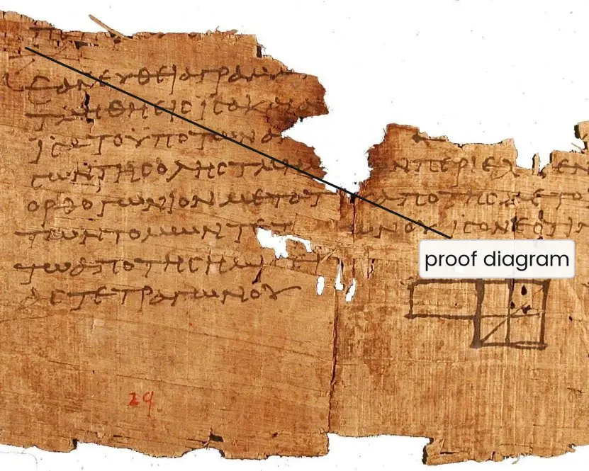
Algorithms are older than computers.
Around 300 BC the Greek mathematician Euclid wrote down, in his Elements, a procedure for finding the greatest common divisor of two numbers; it is still used, unchanged, inside every modern computer.
The word algorithm itself comes from the name of the ninth-century scholar al-Khwarizmi.
In the twentieth century Donald Knuth gathered the whole subject into the many volumes of The Art of Computer Programming, and the phrase "analysis of algorithms" is his.
The photographs below connect the ideas of this unit to the people who shaped them.



1.6.1 Eight applications of data structures in everyday Nepali systems
- Arrays store tabular records. The marks sheet of a TU examination, a list of ward numbers or the days of a Bikram Sambat month are all arrays. An array gives instant access to the i-th element by its index. Because the size is fixed, it suits data whose length is known in advance.
- Stacks undo and go back. When you press the back button in a browser or on the Nagarik App, the last screen you visited is the first one you return to. The same last-in, first-out rule powers the undo command in a word processor. The function call stack of every C program is also a stack.
- Queues keep things fair. A bank token system, a ticket line at a railway counter and the print queue of a college computer lab all serve the oldest request first. Fonepay and ConnectIPS servers also queue payment requests so that none is lost during a busy festival evening. A queue guarantees first come, first served.
- Linked lists grow without waste. A music playlist or the list of open windows can grow and shrink while the program runs. Inserting a node needs only a few pointer changes and no shifting of other items. This makes linked lists suitable when the number of items is not known beforehand.
- Trees show hierarchy. The folders of a computer, the organisation chart of Tribhuvan University (the university, faculties, campuses, departments) and the HTML of a web page are trees. A binary search tree also finds a name among thousands in about a dozen comparisons. Trees combine hierarchy with fast searching.
- Graphs model connections. A road map of the Kathmandu valley, the network of Nepal Telecom towers and the friends of a social-media user are graphs. Route finders such as the one used by ride-hailing apps run shortest-path algorithms on a graph. Whenever the question is "how are these things connected", a graph is the answer.
- Hash tables give instant lookup. A login system finds your account from your username, and a government portal finds a record from a citizenship number, without scanning every record. A hash function converts the key into a table position in one step. Average lookup time is therefore almost constant.
- Priority queues serve the most urgent first. An emergency ward triages patients by severity, not by arrival time, and an operating system runs the highest-priority process first. A heap implements this efficiently, so the most urgent item can be removed in logarithmic time. This is the structure behind scheduling and event simulation.
Formula and fact sheet
- Data structure = data + relationships + operations. ADT = operations without implementation.
- Linear: array, list, stack, queue. Non-linear: tree, graph.
- Growth order: 1 ≪ log n ≪ n ≪ n log n ≪ n² ≪ 2ⁿ ≪ n!.
- Σ 1..n = n(n+1)/2.
Chapter summary
- A data structure organises data for efficient operations; an algorithm is a finite, unambiguous procedure.
- Structures are classified as primitive/non-primitive, linear/non-linear, static/dynamic.
- An ADT specifies behaviour only, so implementations can be swapped.
- The right structure changes cost from linear to logarithmic or constant; Big-O is the common yardstick.
Practice
- Define data structure and algorithm. State two differences.
- Classify: array, stack, tree, graph,
int, linked list. - What is an ADT? Give the ADT of a queue (data, operations, rules).
- Why is a linked list called dynamic while an array is static?
- Which structure would you choose forabrowser back button,ba printer spooler,ca family tree,dphone book lookup by name? Justify.
- Count the steps of summing 1..n by a loop versus by formula, and give the Big-O of each.
- If an algorithm takes 3n² + 5n + 7 steps, what is its Big-O?
- How many comparisons does binary search need, at most, to search 1,000,000 sorted items?
Answers and worked solutions
1. A data structure is a way of organising data with its operations; an algorithm is a finite sequence of steps to solve a problem. The structure holds data; the algorithm acts on it.
2. Array: non-primitive, linear, static. Stack: non-primitive, linear, dynamic or static by implementation. Tree and graph: non-primitive, non-linear. int: primitive. Linked list: non-primitive, linear, dynamic.
3. Queue ADT: data = items in arrival order; operations = enqueue (add at rear), dequeue (remove from front), front, isEmpty, isFull; rule = first in, first out; dequeue on empty is underflow.
4. A linked list allocates each node when needed (malloc) and frees it when done, so its size follows the data. An array size is fixed at declaration.
5.(a) Stack, last page visited is first to return.(b) Queue, first job submitted prints first.(c) Tree, one parent to many children.(d) Hash table or sorted array with binary search, fast key lookup.
6. Loop: n additions → O(n). Formula: one multiplication, one addition, one division → O(1).
7. Drop the constants and lower terms: O(n²).
8. ⌈log₂ 1,000,000⌉ ≈ 20 comparisons (2²⁰ = 1,048,576).
Model answers (5 and 10 marks)
Q1. Define data structure and explain its classification. (5 marks)
A data structure is a systematic way of organising and storing data in memory so that the operations a program needs, such as insertion, deletion, searching and traversal, can be done efficiently.
An algorithm is the finite sequence of steps that works on that data. The two always go together: a good algorithm on a poor structure is still slow.
Data structures are classified in the following way (Figure 1.1).
- Primitive structures are built into the language:
int,char,float,doubleand pointers. The machine understands them directly. - Non-primitive structures are built from primitive ones. They are divided into linear structures (array, stack, queue, linked list), in which items form one sequence, and non-linear structures (tree, graph), in which one item may be connected to many.
- By memory use they are also static (size fixed at compile time, such as an array) or dynamic (size changes at run time, such as a linked list).
For example, a marks sheet of 40 students is naturally an array, while the folders of a college file server form a tree. Choosing the right structure is the first design decision of any program.
Q2. What is an Abstract Data Type? Explain with the example of a stack. (5 marks)
An Abstract Data Type (ADT) is a mathematical description of a data structure in terms of its data, its operations and the rules those operations obey, without saying how it is implemented in memory.
It tells the user what the structure does and hides how it does it.
This hiding is called abstraction and it gives two benefits: the user cannot damage the internals, and the implementation can be changed without changing the programs that use it (Figure 1.2).
The Stack ADT has the following definition.
- Data: an ordered collection of items with one end called the top.
- Operations:
push(x)adds x at the top,pop()removes and returns the top item,peek()reads the top without removing it,isEmpty()andisFull()test the state. - Rule: last in, first out (LIFO). Popping an empty stack is an underflow; pushing onto a full stack is an overflow.
The same ADT can be implemented with an array and an integer top (Unit 2) or with a linked list whose head is the top (Unit 5). A program that only calls push and pop works with both.
In C the usual way to build an ADT is a struct plus a set of functions that receive a pointer to it.
Q3. Explain data structure, its types and importance, and describe how the efficiency of an algorithm is judged. (10 marks)
Introduction. Programs store data and process it. A data structure organises the data so that processing is fast and simple; an algorithm is the procedure that does the processing. Together, in the words of Niklaus Wirth, algorithms plus data structures make programs.
Classification. Figure 1.1 shows that data structures are primitive or non-primitive, the latter being linear (array, stack, queue, linked list) or non-linear (tree, graph), and static or dynamic according to when their size is fixed.
Abstract Data Type. Each structure is specified as an ADT, meaning data, operations and rules without implementation detail, so that the interface stays stable while the implementation may change (Figure 1.2).
Why the choice matters. To find one roll number among 1,000,000 sorted records, linear search needs up to 1,000,000 comparisons, while binary search needs at most 20.
The same data held in an unsorted linked list cannot be searched by halving at all. The structure therefore decides which algorithms are possible.
Judging efficiency. An algorithm is judged by its time complexity (how many basic steps it takes as the input size n grows) and its space complexity (how much extra memory it uses).
We count steps instead of seconds because seconds depend on the machine. We keep only the dominant term, so 3n squared plus 5n plus 7 is written O(n squared).
Figure 1.3 shows the effect: for n = 1,000,000 an O(\log n) method needs about 20 steps but an O(n squared) method needs 10 to the power 12, which is about 11.6 days at one microsecond per step.
| Structure | Access by position | Search | Insert at end | Best use |
|---|---|---|---|---|
| Array | O(1) | O(n); O(\log n) if sorted | O(1) if space | Fixed tables |
| Linked list | O(n) | O(n) | O(1) with tail pointer | Growing lists |
| Stack / queue | top or ends only | O(n) | O(1) | Undo, scheduling |
| Binary search tree | O(\log n) on average | O(\log n) on average | O(\log n) on average | Ordered data |
| Hash table | by key | O(1) on average | O(1) on average | Fast lookup |
Conclusion. A data structure is chosen by asking which operations are most frequent and what cost is acceptable.
Understanding structures, ADTs and Big-O together lets a programmer write software that stays fast as data grows, such as a results system that must serve every TU student at once.