Unit 4 · 10 teaching hours · 49 min read
The Network Layer: Addressing and Routing
What the syllabus asks for 8
- Network layer services
- The IPv4 datagram
- IPv4 addressing
- Subnetting, VLSM and supernetting
- Supporting protocols
- IPv6
- Routing: concepts
- Seeing the ideas: addresses, routes and the boxes that follow them
The network layer is what turns a collection of LANs into an internet.
Its two jobs are forwarding (moving a packet from an input port of a router to the right output port, in nanoseconds) and routing (working out, by algorithm, which output port is right for each destination).
The first needs an addressing scheme that can be summarised; the second needs an algorithm that every router can run on partial information.
This unit does the arithmetic of IPv4 subnetting (checked with Python's ipaddress module), then runs Dijkstra and Bellman–Ford on one network and compares the results.
- Network layer services, datagram versus virtual-circuit service, router architecture.
- IPv4 header, classful and classless addressing, subnetting, VLSM, supernetting, fragmentation.
- ARP, ICMP, DHCP and NAT; IPv6 addressing and transition.
- Routing algorithms: link state (Dijkstra) and distance vector (Bellman–Ford), count-to-infinity, RIP, OSPF, BGP.
4.1 Network layer services
The network layer carries a packet from source host to destination host across many links.
It provides logical addressing, routing, fragmentation and (in the Internet) a best-effort, connectionless service: no guarantee of delivery, order or delay. Reliability is left to TCP at the edges (the end-to-end argument).
A datagram network (IP) forwards every packet independently by its destination address; a virtual-circuit network (ATM, MPLS) sets up a path first and forwards by a short label.
Router architecture. A router has input ports (receive, look up the destination in the forwarding table), a switching fabric (memory, bus or crossbar) and output ports (queue, schedule, transmit).
Queues form when packets arrive faster than they can leave; when buffers fill, packets are dropped. The control plane (routing protocols) builds the table; the data plane forwards.
4.2 The IPv4 datagram
| Field | Bits | Purpose |
|---|---|---|
| Version | 4 | 4 |
| IHL | 4 | header length in 32-bit words (5 = 20 bytes) |
| DSCP/ECN | 8 | priority, congestion notification |
| Total length | 16 | header + data in bytes, at most 65,535 |
| Identification | 16 | which datagram a fragment belongs to |
| Flags | 3 | DF (don't fragment), MF (more fragments) |
| Fragment offset | 13 | position of data in units of 8 bytes |
| TTL | 8 | hop limit, decremented at each router; at 0 the packet is discarded |
| Protocol | 8 | 6 = TCP, 17 = UDP, 1 = ICMP |
| Header checksum | 16 | over the header only (Unit 3) |
| Source / destination address | 32 + 32 | |
| Options | 0–40 bytes | rarely used |
Fragmentation
Each link has a maximum transmission unit (MTU); Ethernet's is 1500 bytes.
If a datagram is larger than the outgoing MTU, a router splits it into fragments, each with its own header, the same identification and the MF flag set on all but the last.
Offsets are in 8-byte units, so every fragment's data except the last is a multiple of 8 bytes.
The datagram has a 20-byte header and 4000 bytes of data. Each fragment may carry 1500 − 20 = 1480 bytes of data (1480 is divisible by 8).
| Fragment | Total length | Data | Offset field | MF |
|---|---|---|---|---|
| 1 | 1500 | 1480 | 0 | 1 |
| 2 | 1500 | 1480 | 185 (= 1480 / 8) | 1 |
| 3 | 1060 | 1040 | 370 | 0 |
Only the destination reassembles; if one fragment is lost the entire datagram is lost, so modern hosts use path MTU discovery (DF set, ICMP "fragmentation needed" returns) instead of fragmenting.
4.3 IPv4 addressing
An IPv4 address has 32 bits written as four decimal bytes (dotted decimal), for example 192.168.10.77. There are 2³² = 4,294,967,296 addresses. An address has a network part (prefix) and a host part; every interface of a host or router has its own address.
Classful addressing (historic)
| Class | First bits | First byte | Default mask | Hosts per network |
|---|---|---|---|---|
| A | 0 | 1–126 | /8 | 16,777,214 |
| B | 10 | 128–191 | /16 | 65,534 |
| C | 110 | 192–223 | /24 | 254 |
| D | 1110 | 224–239 | — | multicast |
| E | 1111 | 240–255 | — | reserved |
Classful addressing wasted space (a company needing 300 hosts took a class B with 65,534), so it was replaced in 1993 by CIDR.
Special and private addresses
- Private (RFC 1918, not routed on the Internet): 10.0.0.0/8, 172.16.0.0/12 (172.16–172.31), 192.168.0.0/16.
- Loopback 127.0.0.0/8 (127.0.0.1 is "this host"); link-local 169.254.0.0/16 (self-assigned when DHCP fails); this network 0.0.0.0; limited broadcast 255.255.255.255; shared address space 100.64.0.0/10 (carrier-grade NAT).
- Within any subnet the all-zeros host part is the network address and the all-ones host part is the directed broadcast address; neither can be given to a host.
CIDR notation
Classless Inter-Domain Routing writes an address with a prefix length: a.b.c.d/n means the first n bits are the network part. The mask is n ones followed by 32 − n zeros. A /n block has 2^{32-n} addresses and 2^{32-n} − 2 usable hosts.
| Prefix | Mask | Addresses | Usable hosts |
|---|---|---|---|
| /24 | 255.255.255.0 | 256 | 254 |
| /25 | 255.255.255.128 | 128 | 126 |
| /26 | 255.255.255.192 | 64 | 62 |
| /27 | 255.255.255.224 | 32 | 30 |
| /28 | 255.255.255.240 | 16 | 14 |
| /29 | 255.255.255.248 | 8 | 6 |
| /30 | 255.255.255.252 | 4 | 2 |
Finding network, broadcast and range
Method: write the mask, AND it with the address to get the network address; set all host bits to 1 for the broadcast address; usable hosts lie in between.
A shortcut: find the interesting octet, compute the block size = 256 − mask value in that octet, and the network address is the nearest multiple of the block size not above the address.
| Address | Network | Mask | Broadcast | First–last host | Hosts |
|---|---|---|---|---|---|
| 192.168.10.77/26 | 192.168.10.64 | 255.255.255.192 | 192.168.10.127 | 192.168.10.65 – 192.168.10.126 | 62 |
| 172.16.5.130/20 | 172.16.0.0 | 255.255.240.0 | 172.16.15.255 | 172.16.0.1 – 172.16.15.254 | 4094 |
| 10.1.2.3/8 | 10.0.0.0 | 255.0.0.0 | 10.255.255.255 | 10.0.0.1 – 10.255.255.254 | 16,777,214 |
| 200.10.20.0/30 | 200.10.20.0 | 255.255.255.252 | 200.10.20.3 | 200.10.20.1 – 200.10.20.2 | 2 |
For 192.168.10.77/26 the block size is 256 − 192 = 64; 77 lies in the block starting at 64, so the network is 192.168.10.64 and the broadcast is 64 + 63 = 127.
For 172.16.5.130/20 the interesting octet is the third: mask 240, block size 16; 5 lies in the block starting at 0, so the network is 172.16.0.0 and the broadcast is 172.16.15.255.
4.4 Subnetting, VLSM and supernetting
Subnetting borrows bits from the host part to create several smaller networks, so one block can serve several LANs. To get N equal subnets borrow ⌈log₂ N⌉ bits.
Six subnets need ⌈log₂ 6⌉ = 3 bits, so the new prefix is /27 and there are 8 subnets (two spare) with 2⁵ − 2 = 30 hosts each: 192.168.1.0, .32, .64, .96, .128, .160, .192 and .224 (all /27). Subnet 3 (index 2) is 192.168.1.64/27: hosts .65–.94, broadcast .95.
Variable-length subnet masks (VLSM) give each LAN a block of the right size.
Procedure: sort requirements from largest to smallest; for each, find the smallest block with at least hosts + 2 addresses; allocate blocks one after another from the start of the address space, keeping each aligned to its own size.
Requirements: Sales 100 hosts, Engineering 50, Admin 25, and a router-to-router WAN link with 2.
| LAN | Hosts needed | Block | Usable hosts | Range | Broadcast |
|---|---|---|---|---|---|
| Sales | 100 | 10.0.0.0/25 | 126 | 10.0.0.1 – 10.0.0.126 | 10.0.0.127 |
| Engineering | 50 | 10.0.0.128/26 | 62 | 10.0.0.129 – 10.0.0.190 | 10.0.0.191 |
| Admin | 25 | 10.0.0.192/27 | 30 | 10.0.0.193 – 10.0.0.222 | 10.0.0.223 |
| WAN link | 2 | 10.0.0.224/30 | 2 | 10.0.0.225 – 10.0.0.226 | 10.0.0.227 |
Used: 128 + 64 + 32 + 4 = 228 of 256 addresses; 10.0.0.228 – 10.0.0.255 stays free for growth. If a naive equal split had been used, a /25 for each of the four LANs would have needed 512 addresses.
Supernetting (route aggregation) does the reverse: combine contiguous blocks into one shorter prefix so that a router needs a single table entry.
The four /24 networks 192.168.0.0 to 192.168.3.0 aggregate to 192.168.0.0/22 (they must be contiguous, a power-of-two count, and the first must be aligned on the block boundary).
ISPs aggregate customer blocks, which keeps the Internet's global routing table manageable.
Longest-prefix match
When several table entries match a destination, the router uses the one with the longest prefix.
With the table 0.0.0.0/0 → default, 10.0.0.0/8 → R1, 10.1.0.0/16 → R2 and 10.1.2.0/24 → R3: destination 10.1.2.9 matches /8, /16 and /24 and goes to R3; 10.1.9.9 matches /8 and /16 and goes to R2; 10.9.9.9 goes to R1; 8.8.8.8 matches only the default route.
4.5 Supporting protocols
ARP and RARP
ARP maps an IP address on the local network to a MAC address (Unit 3). To reach a host outside its subnet, a host ARPs for the default gateway's MAC and sends the frame there with the destination IP of the far host.
At each router the frame's MAC addresses change but the packet's IP addresses stay the same.
ICMP
ICMP carries errors and diagnostics inside IP packets (protocol number 1). Common types: echo request/reply (8/0, the basis of ping), destination unreachable (3), time exceeded (11) and redirect (5).
ping measures round-trip time; traceroute sends probes with TTL = 1, 2, 3, … and records the "time exceeded" replies of successive routers to list the path.
DHCP
A new host has no address, so DHCP (UDP ports 67 server, 68 client) gives it one through four messages: Discover (broadcast from 0.0.0.0 to 255.255.255.255), Offer (server proposes an address, mask, gateway, DNS, lease time), Request (client accepts one offer) and Ack.
The address is leased for a time and renewed halfway through. In a home network the Wi-Fi router is the DHCP server and usually hands out 192.168.1.x or 192.168.0.x addresses.
NAT
Network address translation lets many hosts with private addresses share one public address. The NAT router keeps a table mapping (private IP, private port) to (public IP, public port).
| Direction | Source before → after | Table entry |
|---|---|---|
| Outbound | 192.168.1.10:51000 → 202.79.1.5:40001 | created |
| Outbound | 192.168.1.11:51000 → 202.79.1.5:40002 | created (a different public port for the second host) |
| Inbound reply to :40001 | destination → 192.168.1.10:51000 | looked up |
NAT conserved IPv4 addresses but breaks end-to-end addressing: servers behind NAT need port forwarding, and peer-to-peer apps need traversal tricks (STUN, relays). Many mobile networks use carrier-grade NAT with the 100.64.0.0/10 range.
4.6 IPv6
IPv4's 2³² addresses ran out (IANA's last block was assigned in 2011; APNIC's pool in 2011). IPv6 has 128-bit addresses: 2¹²⁸ ≈ 3.403 × 10³⁸ of them.
Written as eight groups of four hex digits; leading zeros in a group may be dropped and one run of all-zero groups may be replaced by "::". For example, 2001:0db8:0000:0000:0000:ff00:0042:8329 compresses to 2001:db8::ff00:42:8329.
| Type | Prefix | Note |
|---|---|---|
| Global unicast | 2000::/3 | routable on the Internet |
| Link-local | fe80::/10 | automatic on every interface, never routed |
| Unique local | fc00::/7 | the private equivalent |
| Multicast | ff00::/8 | replaces broadcast |
| Loopback | ::1/128 |
An end site normally gets a /48 (65,536 subnets of /64, since 2^{64-48} = 65,536) and every LAN is a /64.
A host can build its own interface identifier by EUI-64: take the MAC 00:1A:2B:3C:4D:5E, insert FF:FE in the middle (00:1A:2B:FF:FE:3C:4D:5E) and flip the universal/local bit (the second-lowest bit of the first byte) to get 021A:2BFF:FE3C:4D5E, so the link-local address is fe80::21a:2bff:fe3c:4d5e.
(Privacy extensions use random identifiers instead.)
Header. The IPv6 header is a fixed 40 bytes: version, traffic class, flow label, payload length, next header, hop limit, source and destination.
There is no header checksum, no fragmentation by routers (only the source may fragment, using an extension header) and options live in extension headers.
Autoconfiguration (SLAAC) uses router advertisements; Neighbor Discovery (ICMPv6) replaces ARP. Transition from IPv4: dual stack (both protocols), tunnelling (IPv6 packets inside IPv4), translation (NAT64/DNS64).
4.7 Routing: concepts
A routing algorithm fills the forwarding tables. Criteria: correctness, simplicity, robustness, stability, fairness and optimality (the cost can be hops, delay, bandwidth or money).
Algorithms are static (non-adaptive, manual, for small stub networks and default routes) or dynamic (adaptive: they react to topology changes).
The two classic dynamic families are link-state (every router learns the whole map and computes shortest paths) and distance-vector (every router tells its neighbours its table).
The example network used below has six routers; the link costs are A–B 2, A–C 5, A–D 1, B–C 3, B–D 2, C–D 3, C–E 1, C–F 5, D–E 1, E–F 2.
4.7.1 Link-state routing and Dijkstra
Each router measures the cost to neighbours, floods a link-state packet to all routers, assembles the same map, and runs Dijkstra's shortest-path algorithm to build a tree rooted at itself: keep a set of finalised nodes; repeatedly finalise the unfinalised node with the least tentative distance and relax its neighbours (if d(u) + w(u,v) < d(v) update d(v) and the predecessor).
| Finalised | A | B | C | D | E | F | Action |
|---|---|---|---|---|---|---|---|
| start | 0 | ∞ | ∞ | ∞ | ∞ | ∞ | |
| A | 0 | 2 (A) | 5 (A) | 1 (A) | ∞ | ∞ | relax A's neighbours |
| D (1) | 0 | 2 (A) | 4 (D) | 1 | 2 (D) | ∞ | via D: C 1 + 3 = 4 < 5; E = 2; B 1 + 2 = 3 is not < 2 |
| B (2) | 0 | 2 | 4 (D) | 1 | 2 (D) | ∞ | via B: C 2 + 3 = 5, no change |
| E (2) | 0 | 2 | 3 (E) | 1 | 2 | 4 (E) | via E: C 2 + 1 = 3 < 4; F 2 + 2 = 4 |
| C (3) | 0 | 2 | 3 | 1 | 2 | 4 (E) | via C: F 3 + 5 = 8, no change |
| F (4) | 0 | 2 | 3 | 1 | 2 | 4 | done |
Order of finalisation: A, D, B, E, C, F. The shortest path to F is A → D → E → F (cost 4); to C it is A → D → E → C (cost 3). A's forwarding table (next hop): B via B; C, D, E and F all via D.
OSPF is the Internet's main link-state protocol: it floods link-state advertisements, uses cost = reference bandwidth / interface bandwidth (cost 10 for 10 Mbps, 1 for 100 Mbps and for 1 Gbps with the default 100 Mbps reference, which is why the reference is usually raised), divides a network into areas joined at a backbone area 0, and elects a designated router on multi-access LANs.
Convergence is fast, but memory and CPU grow with the map.
4.7.2 Distance-vector routing and Bellman–Ford
Each router keeps a vector of its best-known cost to every destination and periodically sends it to neighbours.
On receiving neighbour v's vector, router u computes d_u(t) = min over neighbours v of [ c(u,v) + d_v(t) ] (the Bellman–Ford equation).
It is simple, needs no map, and is distributed: it uses only local knowledge and neighbour information.
| Round | to B | to C | to D | to E | to F |
|---|---|---|---|---|---|
| 0 (neighbours only) | 2 | 5 | 1 | ∞ | ∞ |
| 1 | 2 | 4 | 1 | 2 | 10 |
| 2 | 2 | 3 | 1 | 2 | 4 |
| 3 | 2 | 3 | 1 | 2 | 4 (no change: converged) |
In round 1 A learns about E through D (1 + 1 = 2), but F only through C's first-round value 5 (5 + 5 = 10); in round 2 E's own vector contains F = 2, giving 2 + 2 = 4. The converged costs equal Dijkstra's (0, 2, 3, 1, 2, 4), as they must.
Count to infinity
Distance vector reacts quickly to good news (a shorter path spreads one hop per round) but slowly to bad news. On a line A – B – C with every link cost 1, B reaches C at cost 1 and A at cost 2.
When the link B–C breaks, B looks for another route and hears from A that A can reach C at cost 2, so B sets its cost to 3 via A; then A, whose route goes via B, updates to 4; B to 5; A to 6, and so on: 3, 4, 5, … until the "infinity" value (16 in RIP) is reached, after 14 exchanges in this example.
Fixes: define a small infinity (16 for RIP), split horizon (never advertise a route back to the neighbour it was learned from), poison reverse (advertise it back with cost infinity) and triggered updates.
Split horizon fixes the two-router loop but not all loops.
4.7.3 RIP, OSPF and BGP
| Protocol | Type | Metric | Scope | Facts |
|---|---|---|---|---|
| RIP v1/v2 | distance vector | hop count, max 15, 16 = unreachable | small networks | updates every 30 s over UDP port 520; v2 carries masks and multicast |
| OSPF | link state | cost | inside one autonomous system (interior) | areas, designated router, fast convergence |
| BGP-4 | path vector | policy; shortest AS-path among other attributes | between autonomous systems (exterior) | runs over TCP port 179; routes carry the list of ASes they cross, which prevents loops |
An autonomous system (AS) is a network under one administration with a common routing policy, identified by an AS number. The Internet uses intra-AS protocols (OSPF, IS-IS, RIP) and inter-AS BGP.
Hierarchical routing keeps tables small and lets each organisation hide its internal structure.
Other routing ideas
Broadcast routing uses flooding, reverse-path forwarding or a spanning tree (a tree over n nodes has n − 1 links: 5 for the six routers above).
Multicast (IGMP between host and router; PIM between routers) sends one copy to many group members along a tree. Mobile IP keeps a mobile node reachable using a home agent and a care-of address.
Congestion at the network layer
If routers receive more than they can forward, queues grow and delay rises sharply as utilisation approaches 100 %; at full buffers packets are dropped.
Responses: admission control, traffic shaping (leaky bucket: output at a fixed rate, bucket overflow is discarded; token bucket: allows bursts up to the bucket size), choke packets, load shedding, and active queue management such as RED, which drops packets randomly before the queue is full to signal senders early. TCP reacts to the drops (Unit 5).
Practising the commands
The first program is a subnet calculator built on Python's standard ipaddress module; it reproduces the tables of this unit.
import ipaddress, math
for c in ["192.168.10.77/26", "172.16.5.130/20", "10.1.2.3/8", "200.10.20.0/30"]:
    n = ipaddress.ip_network(c, strict=False); h = list(n.hosts())
    print(c, n.network_address, n.netmask, n.broadcast_address, h[0], h[-1], n.num_addresses - 2)
print([str(s) for s in ipaddress.ip_network("192.168.1.0/24").subnets(new_prefix=27)])
def vlsm(base, reqs):
    cur = int(ipaddress.ip_network(base).network_address)
    for name, hosts in sorted(reqs, key=lambda x: -x[1]):
        bits = math.ceil(math.log2(hosts + 2)); sn = ipaddress.ip_network((cur, 32 - bits))
        h = list(sn.hosts()); print(name, sn, len(h), h[0], h[-1], sn.broadcast_address); cur += 2 ** bits
vlsm("10.0.0.0/24", [("Sales", 100), ("Eng", 50), ("Admin", 25), ("WAN", 2)])
print(list(ipaddress.collapse_addresses([ipaddress.ip_network("192.168.%d.0/24" % i) for i in range(4)])))
table = [("0.0.0.0/0", "default"), ("10.0.0.0/8", "R1"), ("10.1.0.0/16", "R2"), ("10.1.2.0/24", "R3")]
for ip in ["10.1.2.9", "10.1.9.9", "10.9.9.9", "8.8.8.8"]:
    a = ipaddress.ip_address(ip)
    best = max((ipaddress.ip_network(p) for p, _ in table if a in ipaddress.ip_network(p)), key=lambda n: n.prefixlen)
    print(ip, "->", best, dict(table)[str(best)])
a6 = ipaddress.ip_address("2001:0db8:0000:0000:0000:ff00:0042:8329"); print(a6.compressed)
192.168.10.77/26 192.168.10.64 255.255.255.192 192.168.10.127 192.168.10.65 192.168.10.126 62
172.16.5.130/20 172.16.0.0 255.255.240.0 172.16.15.255 172.16.0.1 172.16.15.254 4094
10.1.2.3/8 10.0.0.0 255.0.0.0 10.255.255.255 10.0.0.1 10.255.255.254 16777214
200.10.20.0/30 200.10.20.0 255.255.255.252 200.10.20.3 200.10.20.1 200.10.20.2 2
['192.168.1.0/27', '192.168.1.32/27', '192.168.1.64/27', '192.168.1.96/27', '192.168.1.128/27', '192.168.1.160/27', '192.168.1.192/27', '192.168.1.224/27']
Sales 10.0.0.0/25 126 10.0.0.1 10.0.0.126 10.0.0.127
Eng 10.0.0.128/26 62 10.0.0.129 10.0.0.190 10.0.0.191
Admin 10.0.0.192/27 30 10.0.0.193 10.0.0.222 10.0.0.223
WAN 10.0.0.224/30 2 10.0.0.225 10.0.0.226 10.0.0.227
[IPv4Network('192.168.0.0/22')]
10.1.2.9 -> 10.1.2.0/24 R3
10.1.9.9 -> 10.1.0.0/16 R2
10.9.9.9 -> 10.0.0.0/8 R1
8.8.8.8 -> 0.0.0.0/0 default
2001:db8::ff00:42:8329
The second program runs Dijkstra and a distance-vector computation on the six-router network, and reproduces the fragmentation table.
import heapq, math
G = {"A": {"B": 2, "C": 5, "D": 1}, "B": {"A": 2, "C": 3, "D": 2}, "C": {"A": 5, "B": 3, "D": 3, "E": 1, "F": 5},
     "D": {"A": 1, "B": 2, "C": 3, "E": 1}, "E": {"C": 1, "D": 1, "F": 2}, "F": {"C": 5, "E": 2}}
def dijkstra(G, s):
    dist = {v: math.inf for v in G}; prev = {}; dist[s] = 0; done = []; pq = [(0, s)]
    while pq:
        d, u = heapq.heappop(pq)
        if u in done: continue
        done.append(u)
        for v, w in G[u].items():
            if d + w < dist[v]: dist[v] = d + w; prev[v] = u; heapq.heappush(pq, (d + w, v))
    return dist, prev, done
dist, prev, order = dijkstra(G, "A"); print(dist); print("order", order)
p = ["F"]
while p[-1] in prev: p.append(prev[p[-1]])
print("path to F", p[::-1])
D = {u: {v: (0 if u == v else math.inf) for v in G} for u in G}
for u in G:
    for v, w in G[u].items(): D[u][v] = w
for rnd in range(1, 5):
    new = {u: dict(D[u]) for u in G}; changed = False
    for u in G:
        for t in G:
            if u != t:
                best = min(G[u][v] + D[v][t] for v in G[u])
                if best < new[u][t]: new[u][t] = best; changed = True
    D = new; print("round", rnd, D["A"])
    if not changed: break
def frag(total, mtu, hdr=20):
    payload = total - hdr; per = (mtu - hdr) // 8 * 8; res = []; off = 0
    while payload > 0:
        sz = min(per, payload); payload -= sz; res.append((sz + hdr, off // 8, 0 if payload == 0 else 1)); off += sz
    return res
print(frag(4020, 1500))
{'A': 0, 'B': 2, 'C': 3, 'D': 1, 'E': 2, 'F': 4}
order ['A', 'D', 'B', 'E', 'C', 'F']
path to F ['A', 'D', 'E', 'F']
round 1 {'A': 0, 'B': 2, 'C': 4, 'D': 1, 'E': 2, 'F': 10}
round 2 {'A': 0, 'B': 2, 'C': 3, 'D': 1, 'E': 2, 'F': 4}
round 3 {'A': 0, 'B': 2, 'C': 3, 'D': 1, 'E': 2, 'F': 4}
[(1500, 0, 1), (1500, 185, 1), (1060, 370, 0)]
4.8 Seeing the ideas: addresses, routes and the boxes that follow them
The network layer is mostly arithmetic on 32-bit numbers and graphs, but it was built by people and runs on real boxes.
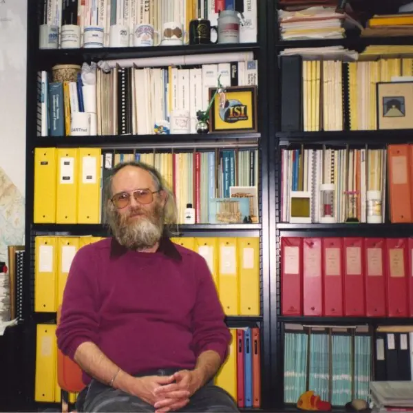
Plate 4.1 shows three of them: Jon Postel, the editor of the early Internet standards, Vint Cerf, a co-designer of TCP/IP, and Edsger Dijkstra, whose shortest-path algorithm every link-state router runs.
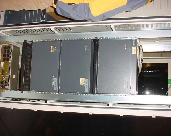
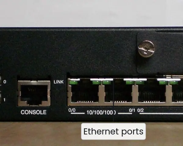
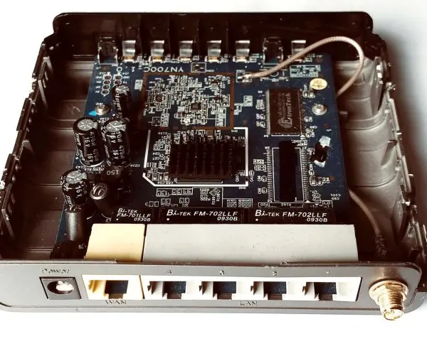
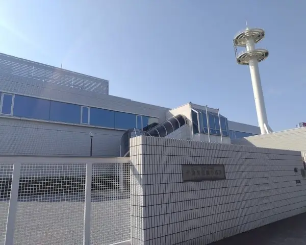
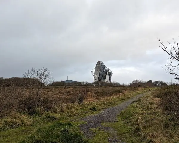
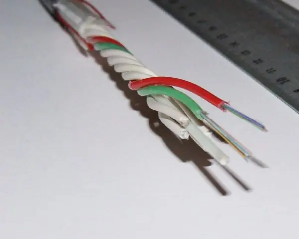
Plate 4.2 shows routers, from a small branch box to a core chassis, and Plate 4.3 shows where packets leave a country: the cable landing station, the satellite dish and the fibre.
The figures that follow compute the unit's examples from the real rules: the header of a real packet, fragmentation, subnet masks, VLSM, longest-prefix match, IPv6 addresses, NAT, DHCP, traceroute, Dijkstra, distance-vector, queueing delay, BGP paths and route aggregation.




4.8.1 Eight uses of network layer technology in Nepal
- Addressing plans for colleges and offices. A college that receives one block of addresses from its ISP divides it into subnets for the office, the labs and the Wi-Fi, using VLSM so that no addresses are wasted (Fig. 4.4). Each lab has its own broadcast domain and its own gateway. Good subnetting also lets the administrator write a firewall rule for one department.
- NAT in every home and mobile network. A family with one broadband line puts a dozen devices behind a single public address, and mobile operators use carrier-grade NAT for millions of phones (Fig. 4.7). IPv4 addresses are scarce, so this is how the country keeps growing. The price is that a home server needs port forwarding.
- DHCP in the home router. Every phone that joins the Wi-Fi gets an address, mask, gateway and DNS server in the four DORA messages (Fig. 4.8). A lease of a few hours lets the router reuse addresses from visitors who have left. When DHCP fails, the phone falls back to a 169.254 address and cannot reach the Internet.
- Diagnosing slow connections with ping and traceroute. A technician who hears that a payment site is slow can run ping to measure delay and traceroute to see which hop adds it (Fig. 4.8). Each hop appears because a router returned an ICMP time-exceeded message. Seeing the delay jump at the hop that leaves the country shows the cause is an international link, not the local network.
- OSPF in ISP and bank networks. An ISP or a bank with many sites runs OSPF so that routers learn the whole map and recompute the shortest paths within a second or two after a link fails (Fig. 4.9). Areas keep the load on small routers low. Link costs are set from bandwidth, so the fibre is preferred over the radio backup.
- BGP to the world. Nepali ISPs buy transit from providers in neighbouring countries and announce their address blocks with BGP (Fig. 4.12). The AS path shows which route is shorter, and policy decides which provider is preferred. A wrong announcement can pull other countries' traffic into the wrong network, so filters are essential.
- Route aggregation by ISPs. An ISP gives customers small blocks from its own large block and announces only the aggregate to the world (Fig. 4.13). This keeps the routing table small and the routers fast. A customer that moves to another ISP must renumber, which is the price of aggregation.
- IPv6 deployment. Mobile and fixed operators in the region are enabling IPv6 so that every device can have its own global address without NAT (Fig. 4.6). A phone builds its link-local address automatically, and a /64 for each LAN removes the need to ration addresses. Dual-stack lets old IPv4-only sites keep working during the transition.
Formula and fact sheet
- Addresses: 2³² IPv4, 2¹²⁸ IPv6. /n block: 2^{32-n} addresses, 2^{32-n} − 2 hosts. Borrow ⌈log₂ N⌉ bits for N subnets.
- Block size = 256 − mask octet. Network = address AND mask. Broadcast = network OR NOT mask.
- Private: 10/8, 172.16/12, 192.168/16. Loopback 127/8. Link-local 169.254/16.
- Fragment offset in 8-byte units; fragment data a multiple of 8 except the last.
- Bellman–Ford: d_u(t) = min_v [c(u,v) + d_v(t)]. Dijkstra: finalise the nearest node, relax edges.
- RIP: hop count, max 15, UDP 520. OSPF: link state, cost = 100 Mbps / bandwidth by default. BGP: path vector, TCP 179.
Chapter summary
- IP is a best-effort, connectionless service; routers forward by longest-prefix match on the destination address and split oversize datagrams into fragments.
- CIDR, subnetting, VLSM and aggregation allow addresses to be allocated and summarised flexibly; ARP, ICMP, DHCP and NAT make IPv4 usable; IPv6 restores the address space.
- Link-state routing (Dijkstra) gives every router the same map; distance-vector routing (Bellman–Ford) shares tables with neighbours and risks count-to-infinity.
- OSPF and RIP route inside an AS, BGP between ASes.
Practice
- Find the network address, broadcast address, range and host count for 192.168.10.77/26 and 172.16.5.130/20.
- Divide 192.168.1.0/24 into at least six equal subnets. Give the prefix, hosts per subnet and the third subnet.
- Design VLSM for 100, 50, 25 and 2 hosts from 10.0.0.0/24.
- Which prefix is needed for a LAN of 500 hosts?
- Aggregate 192.168.0.0/24 to 192.168.3.0/24.
- Longest-prefix match: to where is 10.1.9.9 forwarded with the table in Section 4.4?
- A 4020-byte datagram meets an MTU of 1500. Give each fragment's length, offset and MF.
- Run Dijkstra on the six-router network from A; give the path to F and A's next hops.
- Do three rounds of distance-vector at A and compare with Dijkstra.
- Explain count to infinity, split horizon and poison reverse.
- Describe the four DHCP messages and what NAT does with the port number.
- Compress 2001:0db8:0000:0000:0000:ff00:0042:8329. How many /64 subnets are in a /48?
Answers and worked solutions
1. 192.168.10.77/26: network 192.168.10.64, broadcast 192.168.10.127, hosts .65–.126 (62). 172.16.5.130/20: network 172.16.0.0, broadcast 172.16.15.255, hosts 172.16.0.1–172.16.15.254 (4094).
2. ⌈log₂ 6⌉ = 3 borrowed bits: /27, 8 subnets, 30 hosts each; the third is 192.168.1.64/27 (hosts .65–.94, broadcast .95).
3. Sales 10.0.0.0/25, Engineering 10.0.0.128/26, Admin 10.0.0.192/27, WAN 10.0.0.224/30 (table in Section 4.4).
4. 500 + 2 = 502 addresses need 9 host bits (512), so the prefix is /23 (32 − 9).
5. 192.168.0.0/22.
6. It matches 10.0.0.0/8 and 10.1.0.0/16 (not 10.1.2.0/24); the longest is /16, so R2.
7. (1500, offset 0, MF 1), (1500, offset 185, MF 1), (1060, offset 370, MF 0).
8. Dist: A 0, B 2, C 3, D 1, E 2, F 4; path A → D → E → F; next hops: B via B, everything else via D.
9. Round 1: 2, 4, 1, 2, 10; round 2: 2, 3, 1, 2, 4; round 3 unchanged. The same as Dijkstra.
10. After a failure, two routers keep increasing each other's cost by one (3, 4, 5, … up to 16 in RIP). Split horizon withholds a route from the neighbour it came from; poison reverse advertises it back with infinity so the neighbour does not use it.
11. Discover, Offer, Request, Ack. NAT rewrites the private source address and port to the public address and a unique public port and keeps a table to translate replies back.
12. 2001:db8::ff00:42:8329. A /48 contains 2^{64-48} = 65,536 subnets of /64.
Model answers for Unit 4
Q1. Explain IPv4 addressing, classful addressing and CIDR. For the address 192.168.10.77/26 find the network address, broadcast address and usable host range. (10 marks)
Introduction. An IPv4 address is 32 bits, written as four decimal bytes, and identifies one interface. It has a network part and a host part, and the dividing line decides how many networks and how many hosts per network exist.
Classful addressing (historic). The first bits of the address fixed the split.
| Class | First bits | First byte | Default mask | Hosts per network |
|---|---|---|---|---|
| A | 0 | 1-126 | /8 | 16 777 214 |
| B | 10 | 128-191 | /16 | 65 534 |
| C | 110 | 192-223 | /24 | 254 |
| D | 1110 | 224-239 | none | multicast |
| E | 1111 | 240-255 | none | reserved |
A company needing 300 hosts had to take a class B and waste more than 65 000 addresses, so in 1993 CIDR replaced the classes.
CIDR. The address is written a.b.c.d/n, where the first n bits are the network part and the mask is n ones followed by 32 - n zeros.
A /n block has 2^{32-n} addresses, of which 2^{32-n} - 2 are usable, because the all-zeros host part is the network address and the all-ones host part is the broadcast address.
Private ranges (10.0.0.0/8, 172.16.0.0/12, 192.168.0.0/16) are not routed on the Internet.
Worked example (Fig. 4.3). For 192.168.10.77/26 the mask is 255.255.255.192.
- The interesting octet is the fourth: block size = 256 - 192 = 64.
- 77 lies in the block that starts at 64, so the network address is 192.168.10.64.
- The broadcast address is 64 + 63 = 192.168.10.127.
- The usable hosts run from 192.168.10.65 to 192.168.10.126, which is 62 hosts.
Special addresses. Some addresses have fixed meanings: 127.0.0.1 (loopback, this host), 169.254.0.0/16 (link-local, chosen automatically when DHCP fails), 255.255.255.255 (limited broadcast) and 100.64.0.0/10 (shared space used by carrier-grade NAT).
A host in the same subnet is reached directly by ARP, while any other destination is sent to the default gateway, so the mask also decides what is local.
Conclusion. CIDR lets a block of any power-of-two size be given to a network, which saved the IPv4 space for another two decades and allowed route aggregation.
Q2. Explain VLSM and route aggregation. Divide 10.0.0.0/24 among LANs of 100, 50 and 25 hosts and a 2-host router link. (10 marks)
Introduction. Plain subnetting gives every subnet the same size, which wastes addresses when the LANs differ.
Variable-length subnet masks (VLSM) give each LAN a block of the right size, and route aggregation (supernetting) does the reverse, joining blocks into one shorter prefix.
VLSM procedure.
- List the LANs from largest to smallest.
- For each, find the smallest block with at least hosts + 2 addresses (network and broadcast).
- Allocate the blocks one after another from the start, each aligned to a multiple of its own size.
Worked example (Fig. 4.4).
| LAN | Hosts | Block | Usable hosts | Range | Broadcast |
|---|---|---|---|---|---|
| Sales | 100 | 10.0.0.0/25 | 126 | 10.0.0.1 - 10.0.0.126 | 10.0.0.127 |
| Engineering | 50 | 10.0.0.128/26 | 62 | 10.0.0.129 - 10.0.0.190 | 10.0.0.191 |
| Admin | 25 | 10.0.0.192/27 | 30 | 10.0.0.193 - 10.0.0.222 | 10.0.0.223 |
| WAN link | 2 | 10.0.0.224/30 | 2 | 10.0.0.225 - 10.0.0.226 | 10.0.0.227 |
The blocks use 128 + 64 + 32 + 4 = 228 addresses, and 10.0.0.228 to 10.0.0.255 remains free. An equal split would need a /25 for each of the four LANs, which is 512 addresses and would not fit in the /24.
Route aggregation (Fig. 4.13). Four contiguous /24 networks, 192.168.0.0 to 192.168.3.0, share their first 22 bits, so a router can announce the single prefix 192.168.0.0/22.
The conditions are that the blocks are contiguous, their number is a power of two and the first block is aligned on the block size.
Longest-prefix match (Fig. 4.5). When several routes match, the router uses the one with the longest prefix, so a more specific route overrides the aggregate.
Conclusion. VLSM saves addresses inside an organisation, and aggregation saves routing-table entries outside it. Both depend on addresses being allocated in aligned power-of-two blocks.
Q3. Describe the IPv4 datagram format. How is a 4020 byte datagram fragmented over a link with MTU 1500? (10 marks)
Introduction. The IPv4 datagram is a header of 20 to 60 bytes followed by data. The header (Fig. 4.1) carries everything a router needs to forward the packet.
Main header fields.
- Version and IHL: 4 for IPv4; the header length in 32-bit words (5 means 20 bytes).
- Total length: header plus data in bytes, at most 65 535.
- Identification, flags and fragment offset: these let the destination reassemble fragments; the flags are DF (do not fragment) and MF (more fragments), and the offset counts 8-byte units.
- TTL: the hop limit, decreased by every router; at 0 the packet is discarded, which stops loops and makes traceroute possible.
- Protocol: which upper layer receives the data (6 = TCP, 17 = UDP, 1 = ICMP).
- Header checksum: the Internet checksum over the header only.
- Source and destination addresses: 32 bits each.
Fragmentation (Fig. 4.2). The datagram has a 20-byte header and 4000 bytes of data. With MTU 1500 each fragment can carry 1500 - 20 = 1480 bytes of data, and 1480 is a multiple of 8.
| Fragment | Total length | Data bytes | Offset field | MF |
|---|---|---|---|---|
| 1 | 1500 | 1480 | 0 | 1 |
| 2 | 1500 | 1480 | 185 | 1 |
| 3 | 1060 | 1040 | 370 | 0 |
All fragments have the same identification. Only the destination reassembles them, and if one fragment is lost the entire datagram is lost. Fragmenting also adds two extra headers (40 bytes), so modern hosts set DF and use path MTU discovery instead.
Reassembly. The destination collects all fragments with the same identification, source, destination and protocol, places each at its offset (offset x 8 bytes), and delivers the datagram when the fragment with MF = 0 and all earlier pieces have arrived.
A timer discards the partial datagram if a piece never comes. Because the TTL changes at every router, each router also recomputes the header checksum, which is why the checksum covers only the header and is cheap.
Conclusion. The header gives IP a simple, fast forwarding job, and fragmentation lets one datagram cross links of different MTU at some cost in overhead and reliability.
Q4. Compare link-state and distance-vector routing. Apply Dijkstra's algorithm from router A on the network of Fig. 4.9. (10 marks)
Introduction. A routing algorithm fills the forwarding tables. The two main families differ in what a router knows and what it sends.
Link-state routing. Each router measures the cost to its neighbours, floods this information to all routers, builds the complete map and runs Dijkstra's algorithm to compute shortest paths. OSPF and IS-IS work like this.
Distance-vector routing. Each router keeps a vector of costs to every destination and sends it only to neighbours, who apply the Bellman-Ford rule d(u) = min of c(u,v) + d(v). RIP works like this.
Dijkstra from A. The links are A-B 2, A-C 5, A-D 1, B-C 3, B-D 2, C-D 3, C-E 1, C-F 5, D-E 1, E-F 2.
- Finalise A (0); the tentative costs are B 2, C 5, D 1.
- Finalise D (1); via D: C = 4, E = 2.
- Finalise B (2); via B nothing improves (C would be 5).
- Finalise E (2); via E: C = 3, F = 4.
- Finalise C (3); then F (4).
The order is A, D, B, E, C, F, with costs B 2, C 3, D 1, E 2, F 4. The shortest path to F is A, D, E, F. A's next hops are B for B and D for everything else.
| Point | Link state | Distance vector |
|---|---|---|
| Knowledge | whole map | only neighbours' vectors |
| Information sent | own links, flooded to all | whole vector, to neighbours |
| Algorithm | Dijkstra | Bellman-Ford |
| Convergence | fast | slow, count to infinity |
| Memory and CPU | more | less |
| Example | OSPF, IS-IS | RIP |
Check of the answer. Distance vector reaches the same costs: after round 2 router A holds 2, 3, 1, 2, 4 for B, C, D, E and F, and round 3 changes nothing (Fig. 4.10).
The tree of shortest paths from A has five links, one fewer than the number of routers, so every router is reached once and no loops exist.
Conclusion. Link state converges quickly and scales with areas, and distance vector is simpler but slower to react to bad news. Both give the same costs when converged (Fig. 4.10).
Q5. What is the count-to-infinity problem and how is it reduced? (5 marks)
Distance-vector routing spreads good news fast but bad news slowly. In the line A - B - C with all costs 1, B reaches C at cost 1 and A at cost 2.
- The failure. The link B-C breaks. B looks for another route and hears from A that A can reach C at cost 2, so B sets its cost to 3 via A.
- The loop. A's route to C goes through B, so A raises its cost to 4; B then raises to 5, A to 6, and so on.
- The end. The costs rise by one per exchange until they reach the value taken as infinity, 16 in RIP, after 14 exchanges (Fig. 4.10). During this time packets for C loop between A and B.
- Remedies. Defining a small infinity (16) limits the damage; split horizon stops a router advertising a route back to the neighbour it learned it from; poison reverse advertises it back with cost infinity; triggered updates and hold-down timers send bad news at once.
- Limit. These tricks fail for some loops through three or more routers, which is why link-state protocols are preferred in large networks.
Q6. Explain NAT with an example. State its advantages and disadvantages. (5 marks)
Network address translation lets many hosts with private addresses share one public address. The NAT router rewrites the source address and port of each outgoing packet and remembers the mapping in a table (Fig. 4.7).
- Outbound. Host 192.168.1.10 sends from port 51000; the router rewrites the source to 202.79.1.5:40001 and creates a table entry.
- Second host. Host 192.168.1.11 also uses port 51000; the router assigns 40002, so the two flows stay separate.
- Inbound. A reply to 202.79.1.5:40002 is looked up and sent to 192.168.1.11:51000.
- Advantages. It saves public addresses, hides the internal structure, and lets a network change ISP without renumbering the inside. Unsolicited packets find no entry and are dropped.
- Disadvantages. It breaks end-to-end addressing, so servers need port forwarding; peer-to-peer and some voice applications need traversal methods; and the router must keep state for every flow. IPv6 removes the need for NAT.
Q7. Explain how DHCP and ICMP (ping and traceroute) work. (5 marks)
DHCP gives a new host its address automatically. It works in four messages, DORA (Fig. 4.8), using UDP ports 67 (server) and 68 (client).
- Discover: the client broadcasts from 0.0.0.0 to 255.255.255.255.
- Offer: a server proposes an address, mask, gateway, DNS server and lease time.
- Request: the client broadcasts that it accepts one offer.
- Ack: the server confirms; the lease is renewed halfway through.
ICMP carries errors and diagnostics inside IP packets (protocol 1). ping sends echo requests (type 8) and measures the time of the echo replies (type 0).
traceroute sends probes with TTL = 1, 2, 3 and so on; each router that reduces the TTL to 0 discards the packet and returns a time-exceeded message (type 11), so the addresses and delays of the routers on the path are listed one by one.
A star in the output means a router did not answer, not that the path is broken.
Other common ICMP messages are destination unreachable (type 3), used also for path MTU discovery, and redirect (type 5), which tells a host about a better gateway.
Q8. Compare IPv4 and IPv6. Explain IPv6 address notation, types and the transition methods. (10 marks)
Introduction. IPv4 has only 2^{32} (about 4.3 billion) addresses, and its pool ran out in 2011. IPv6 has 128-bit addresses, which is 2^{128} = 3.4 x 10^{38}, and simplifies the header.
Notation. An IPv6 address is eight groups of four hex digits. Leading zeros in a group may be dropped, and one run of all-zero groups may be replaced by a double colon: 2001:0db8:0000:0000:0000:ff00:0042:8329 becomes 2001:db8::ff00:42:8329 (Fig. 4.6).
Address types.
| Type | Prefix | Note |
|---|---|---|
| Global unicast | 2000::/3 | routable on the Internet |
| Link-local | fe80::/10 | automatic on every interface |
| Unique local | fc00::/7 | private equivalent |
| Multicast | ff00::/8 | replaces broadcast |
| Loopback | ::1/128 | this host |
A site normally receives a /48 and every LAN is a /64. A host can form its own interface identifier with EUI-64: insert FF:FE into the MAC address and flip one bit, so 00:1A:2B:3C:4D:5E gives fe80::21a:2bff:fe3c:4d5e.
Comparison.
| Feature | IPv4 | IPv6 |
|---|---|---|
| Address | 32 bits | 128 bits |
| Header | 20-60 bytes, checksum | fixed 40 bytes, no checksum |
| Fragmentation | routers and source | source only |
| Configuration | DHCP, manual | SLAAC and DHCPv6 |
| Address resolution | ARP | Neighbor Discovery (ICMPv6) |
| Broadcast | yes | no (multicast) |
| NAT | widely needed | not needed |
Transition. Three methods let the two protocols coexist: dual stack (hosts run both), tunnelling (IPv6 packets carried inside IPv4) and translation (a gateway converts between them, for example NAT64).
Header differences. The IPv6 header is a fixed 40 bytes with version, traffic class, flow label, payload length, next header, hop limit and the two 128-bit addresses.
It has no header checksum (the link layer and TCP or UDP already check) and no IHL, and routers never fragment: only the source does, using an extension header, so it must discover the path MTU first.
Options live in extension headers that most routers do not inspect, which makes forwarding faster. Hosts configure themselves with router advertisements (SLAAC) and find neighbours with ICMPv6 instead of ARP.
Conclusion. IPv6 solves the address shortage and restores end-to-end addressing, and the transition will continue for many years with dual-stack as the usual path.
Q9. Compare RIP, OSPF and BGP. (5 marks)
An autonomous system (AS) is a group of networks under one administration with one routing policy. Protocols inside an AS are interior, and protocols between ASes are exterior (Fig. 4.12).
- RIP is a distance-vector protocol with the hop count as its metric. The largest usable value is 15, and 16 means unreachable. It sends updates every 30 seconds over UDP port 520 and suits small networks.
- OSPF is a link-state protocol. It floods link-state advertisements, uses a cost based on bandwidth, divides a large network into areas joined at area 0, and elects a designated router on LANs. It converges fast and is the usual interior protocol.
- BGP is a path-vector protocol between ASes. It runs over TCP port 179, and each route carries the list of ASes it has crossed, which prevents loops and shows the length of the path. Policy decides the choice among routes.
- Choice. A company uses OSPF inside; an ISP uses OSPF or IS-IS inside and BGP to its customers and to other ISPs.