Unit 7 · 5 teaching hours · 27 min read
Curves, Surfaces and Computer Animation
What the syllabus asks for 6
- Representing curves
- Bézier curves
- B-spline curves
- Surfaces and 3D models
- Computer animation
- Seeing the ideas: curves, continuity, easing and morphing
Lines and circles cannot draw the outline of the letter "ग", the body of a car or the path of a character's hand.
Designers need curves they can shape with a few handles and that join smoothly: the Bézier and B-spline curves behind every font, vector-drawing program and animation-path editor.
And once shapes can be described, animation changes them over time: keyframes fix the important poses and the computer fills in the frames between.
This unit gives the mathematics of Bézier and B-spline curves with computed points, surface representation, and the techniques and arithmetic of computer animation: interpolation, easing, morphing, frame rates and storage.
- Bézier curves: Bernstein basis, the de Casteljau construction, end tangents, subdivision; the uniform cubic B-spline.
- Polygon meshes and the idea of curved surfaces; fractals and subdivision in outline.
- Animation: keyframes, in-betweening, linear and eased interpolation, morphing, the twelve principles.
- Frame rates, storage arithmetic and animation tools and file formats.
7.1 Representing curves
A curve can be given explicitly (y = f(x), which cannot represent a vertical tangent or a circle), implicitly (f(x, y) = 0, such as x² + y² = r²) or parametrically (x = x(t), y = y(t)), which is the standard in graphics because it handles any shape and gives a natural direction.
Designers want control points that guide the curve intuitively.
A curve interpolates its control points if it passes through them (Lagrange or Hermite curves, which can oscillate), or approximates them if it is merely pulled towards them (Bézier and B-splines, which are smooth and predictable).
Two curve segments joined at a point have C⁰ continuity if the positions match, C¹ if the tangents also match and C² if the curvature matches too; G¹ (geometric) only requires tangent directions to match.
7.2 Bézier curves
A Bézier curve of degree n with control points P₀ … Pₙ is B(t) = Σ Bᵢ,ₙ(t) · Pᵢ, 0 ≤ t ≤ 1, where Bᵢ,ₙ(t) = C(n, i) tⁱ (1 − t)ⁿ⁻ⁱ are the Bernstein polynomials.
For the cubic (n = 3): B(t) = (1 − t)³P₀ + 3t(1 − t)²P₁ + 3t²(1 − t)P₂ + t³P₃.
Properties: the curve starts at P₀ and ends at Pₙ, is tangent to the first and last segments of the control polygon, lies inside the convex hull of the control points, and the basis functions are non-negative and sum to 1 (a partition of unity), so each point is a weighted average.
Moving one control point changes the whole curve (no local control); to get more shape, join several cubics rather than raising the degree.
Control points P₀ = (0, 0), P₁ = (1, 3), P₂ = (4, 3), P₃ = (5, 0).
| t | B0 = (1−t)³ | B1 = 3t(1−t)² | B2 = 3t²(1−t) | B3 = t³ | Point B(t) |
|---|---|---|---|---|---|
| 0 | 1.0000 | 0.0000 | 0.0000 | 0.0000 | (0.0000, 0.0000) |
| 0.25 | 0.4219 | 0.4219 | 0.1406 | 0.0156 | (1.0625, 1.6875) |
| 0.5 | 0.1250 | 0.3750 | 0.3750 | 0.1250 | (2.5000, 2.2500) |
| 0.75 | 0.0156 | 0.1406 | 0.4219 | 0.4219 | (3.9375, 1.6875) |
| 1 | 0.0000 | 0.0000 | 0.0000 | 1.0000 | (5.0000, 0.0000) |
At t = 0.5 the weights are 1/8, 3/8, 3/8, 1/8 and the point is (2.500, 2.250), for instance x = (0 + 3·1 + 3·4 + 5)/8 = 20/8 = 2.5 and y = (0 + 9 + 9 + 0)/8 = 2.25.
The end tangents are B′(0) = 3·(P1 − P0) = (3, 9) and B′(1) = 3·(P3 − P2) = (3, -9): the curve leaves P₀ towards P₁ and enters P₃ from P₂.
The checker confirmed the Bernstein form against the de Casteljau form at eleven values of t and the end derivative against a numerical difference.
The de Casteljau algorithm
A numerically stable and geometric way to evaluate B(t): repeatedly interpolate between neighbouring points.
For t = 0.5: the midpoints of P₀P₁, P₁P₂, P₂P₃ are (0.5, 1.5), (2.5, 3), (4.5, 1.5); the midpoints of those are (1.5, 2.25), (3.5, 2.25); and the midpoint of the last two is (2.5, 2.25), which is B(0.5).
The intermediate points are also the control points of the two halves: the left half has control polygon P₀, (0.5, 1.5), (1.5, 2.25), (2.5, 2.25) and the right half (2.5, 2.25), (3.5, 2.25), (4.5, 1.5), P₃.
This is subdivision, used to draw a curve by splitting until the pieces are flat enough to draw as lines, and to compute intersections.
7.3 B-spline curves
A B-spline is a piecewise polynomial that gives local control (moving a control point changes only a few spans) and automatic continuity between pieces: a uniform cubic B-spline has C² continuity everywhere. For four consecutive control points the segment is
B(t) = (1/6) [t³ t² t 1] · [[−1, 3, −3, 1], [3, −6, 3, 0], [−3, 0, 3, 0], [1, 4, 1, 0]] · [P₀, P₁, P₂, P₃]ᵀ.
Unlike a Bézier curve, the B-spline does not pass through its end control points: at t = 0 it is at (P₀ + 4P₁ + P₂)/6 and at t = 1 at (P₁ + 4P₂ + P₃)/6.
Control points (0, 0), (2, 4), (5, 4), (7, 0).
| t | Point on the uniform cubic B-spline segment |
|---|---|
| 0 | (2.1667, 3.3333) |
| 0.25 | (2.8177, 3.7083) |
| 0.5 | (3.5000, 3.8333) |
| 0.75 | (4.1823, 3.7083) |
| 1 | (4.8333, 3.3333) |
At t = 0 the point is (2.1667, 3.3333), which equals (P₀ + 4P₁ + P₂)/6 = (2.1667, 3.3333), and at t = 1 it is (4.8333, 3.3333).
The curve stays well inside the control polygon: smoother, but it neither starts at (0, 0) nor ends at (7, 0).
Adding the next control point shifts the window by one and gives the next segment, which meets this one with matching position, tangent and curvature.
NURBS (non-uniform rational B-splines) add weights and knot spacing to represent exact circles and conics, and are the standard in CAD.
| Bézier | Uniform cubic B-spline | |
|---|---|---|
| Passes through end points | Yes | No |
| Local control | No (global) | Yes |
| Continuity between joined pieces | Must be arranged (C¹ by collinear handles) | C² automatic |
| Typical use | Fonts, vector drawing, easing curves | Smooth paths, CAD (as NURBS) |
7.4 Surfaces and 3D models
Most 3D objects are stored as polygon meshes: lists of vertices, edges and faces (usually triangles), with per-vertex normals and texture coordinates. Meshes are fast to render but need many polygons for smooth shapes.
Parametric surfaces extend curves: a Bézier patch uses a grid of 4 × 4 control points and S(u, v) = Σ Σ Bᵢ(u) Bⱼ(v) Pᵢⱼ. Subdivision surfaces repeatedly refine a coarse mesh into a smooth limit (the method of choice in animated films).
Solid modelling uses constructive solid geometry (CSG) (union, intersection and difference of primitives such as spheres and boxes) and sweeps.
Fractals such as the Koch curve and the Mandelbrot set are generated by repeating a rule at smaller scale; they model coastlines, mountains and clouds with self-similarity.
Procedural modelling and particle systems (fire, smoke, rain) generate geometry with rules and random numbers; 3D scanning and photogrammetry capture real objects.
7.5 Computer animation
Animation creates the illusion of motion by showing a sequence of still images (frames) quickly enough that the eye blends them (persistence of vision).
Film runs at 24 frames per second (fps), television at 25 or 30, games at 30 to 120. Compared with 24 fps, 30 fps has 1.25 times as many frames to produce.
Production stages: storyboarding, modelling, rigging (building a skeleton and controls), animation, lighting and rendering, compositing and sound.
Keyframing. The animator specifies keyframes (extreme poses at chosen times); the computer generates the in-betweens by interpolating each animated parameter (position, rotation, scale, colour).
Linear interpolation gives x(t) = (1 − t)x₀ + t·x₁, a constant speed with abrupt starts and stops that look mechanical. Easing curves give natural acceleration and deceleration.
A common one is the smoothstep function s(t) = 3t² − 2t³, whose slope is zero at both ends. Moving an object from x = 0 to x = 100 in 24 frames:
| Frame | t = f/24 | Linear x = 100t | Ease in-out x = 100(3t²−2t³) |
|---|---|---|---|
| 0 | 0.000 | 0.00 | 0.00 |
| 4 | 0.167 | 16.67 | 7.41 |
| 8 | 0.333 | 33.33 | 25.93 |
| 12 | 0.500 | 50.00 | 50.00 |
| 16 | 0.667 | 66.67 | 74.07 |
| 20 | 0.833 | 83.33 | 92.59 |
| 24 | 1.000 | 100.00 | 100.00 |
At frame 4 the linear motion has already covered 16.67 units but the eased motion only 7.41: it starts slowly. Animators edit these timing curves as Bézier splines in a graph editor.
For rotations, interpolating Euler angles can behave badly (gimbal lock), so systems use quaternions and spherical linear interpolation (slerp) which follow the shortest rotation at constant angular speed.
Morphing transforms one shape into another by interpolating corresponding vertices (shape morphing) while cross-dissolving colours (image morphing, with warped meshes so that the features align).
A triangle with vertices (0, 0), (4, 0), (4, 3) morphed to (1, 1), (6, 1), (3, 6):
| t | Vertex 1 | Vertex 2 | Vertex 3 |
|---|---|---|---|
| 0 | (0.00, 0.00) | (4.00, 0.00) | (4.00, 3.00) |
| 0.25 | (0.25, 0.25) | (4.50, 0.25) | (3.75, 3.75) |
| 0.5 | (0.50, 0.50) | (5.00, 0.50) | (3.50, 4.50) |
| 1 | (1.00, 1.00) | (6.00, 1.00) | (3.00, 6.00) |
At t = 0.5 the vertices are (0.5, 0.5), (5.0, 0.5), (3.5, 4.5), the average of corresponding vertices.
The result depends on which vertex corresponds to which (a mismatch makes the shape twist or collapse), and the number of vertices must match, so morphing tools add vertices to the simpler shape.
Other techniques. Skeletal animation drives a mesh with a hierarchy of bones (with skinning weights blending the vertices); forward kinematics sets joint angles, inverse kinematics finds joint angles that place a hand or foot at a target; motion capture records real performers; physics-based animation simulates cloth, fluids, rigid bodies and particles using equations of motion; procedural animation uses rules (crowds, flocks, boids).
Disney's twelve principles of animation (squash and stretch, anticipation, staging, straight-ahead action and pose-to-pose, follow-through and overlapping action, slow in and slow out, arcs, secondary action, timing, exaggeration, solid drawing and appeal) guide quality in 2D and 3D alike.
Frames, storage and tools
A 90-second clip at 24 fps has 24 × 90 = 2,160 frames.
Uncompressed full-HD frames at 24 bits are 6.22 MB each, so the raw clip would take 2,160 × 6.22 MB = 13.44 GB (12.51 GiB); video compression (H.264, H.265, AV1) reduces this by two orders of magnitude by storing only the differences between frames.
Image sequences (PNG, EXR) are the usual render output; containers such as MP4 hold compressed video; GIF and animated SVG/CSS are used on the web; glTF and FBX carry 3D animated models.
Tools: Blender (free, complete 3D pipeline), Maya, Houdini for 3D; Toon Boom and Krita for 2D; After Effects for motion graphics.
For the web, CSS transitions and the requestAnimationFrame loop apply the same easing curves to interface elements.
7.6 Seeing the ideas: curves, continuity, easing and morphing
Curves and animation are about shape over a parameter: the parameter t along a curve, or the time t along a shot.
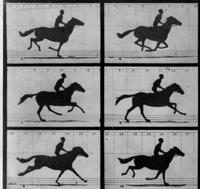
The plate begins with the experiment that proved a galloping horse can be broken into frames, and with the geometric construction that draws a Bézier curve. The figures use the numbers of the worked examples in this unit.


7.6.1 Eight applications of curves and animation
- Fonts for Nepali and English text. Every letter of a digital font, including each Devanagari character, is an outline made of straight lines and Bézier curves. Because the outline is mathematics and not pixels, the letter can be enlarged for a poster or shrunk for a phone without turning jagged. A designer edits only a few control points to change the shape.
- Vector drawing and logos. Programs such as Inkscape and Illustrator let a designer drag Bézier handles to draw logos, maps and icons. The file stays small and prints sharply at any size. A shop signboard in Kathmandu and a mobile-app icon can come from the same drawing.
- Car, aircraft and product design. B-spline and NURBS surfaces give the smooth, flowing bodywork of a car or the wing of an aircraft. The designer moves a control point and only a small region changes, because B-splines have local control. This is why CAD packages use NURBS rather than raw meshes.
- Animation paths and motion design. The path of a camera or a character's hand is a curve with a few control points. The animator reshapes it instead of positioning every frame. Studios use this to produce television advertisements and short films quickly.
- Easing in apps and websites. When a menu slides in or a button grows, easing curves such as smoothstep or a Bézier timing function make the motion feel natural. Both Android and CSS accept a Bézier curve as the timing function. A banking app like those used in Nepal looks calmer and more professional with these small animations.
- Computer games. Characters are animated by skeletons whose bones are rotated between keyframes, and in-between poses are computed in real time. Cameras follow smooth spline paths. Mobile games show a running character at 30 or 60 frames per second this way.
- Education and e-learning videos. Teachers produce explanatory animations in which a diagram is morphed from one stage to the next, such as a triangle changing into another shape or a cell dividing. Pupils follow a process more easily than from a still picture. Online classes made for Nepali schools use this technique.
- Film special effects and medicine. Morphing blends one face or object into another, and motion capture records the movement of real performers. In medicine the beating heart from a scan is animated by interpolating between frames. Both rely on the same idea: keyframes are fixed and the computer fills in between.

Chapter summary
- Parametric curves with control points give designers local, predictable shape control; continuity is described as C⁰, C¹, C².
- Bézier curves use Bernstein weights, pass through the end points, lie in the convex hull and are evaluated by de Casteljau subdivision; the cubic B-spline gives C² continuity and local control but does not pass through the end points.
- 3D shapes are polygon meshes, patches, subdivision surfaces, CSG or procedural models.
- Animation uses keyframes and interpolation; easing (smoothstep 3t² − 2t³) replaces robotic constant speed; morphing interpolates corresponding vertices.
- A 90-second 24 fps full-HD clip is 2,160 frames and 13.44 GB uncompressed.
Practice
- Write the cubic Bézier formula and give B(0.5) for control points (0, 0), (2, 4), (6, 4), (8, 0).
- List four properties of Bézier curves.
- Explain the de Casteljau construction for t = 0.5.
- Why are B-splines preferred over a single high-degree Bézier curve for long curves?
- What is the difference between C¹ and G¹ continuity?
- Compute the smoothstep value at t = 0.25.
- Linearly interpolate the point from (2, 6) at frame 0 to (10, 2) at frame 8; give the position at frame 3.
- Name three principles of animation and explain one.
- Compute the raw size in MB of 10 seconds of 1280 × 720, 24-bit video at 30 fps.
- Differentiate forward and inverse kinematics.
Answers and worked solutions
1. B(t) = (1 − t)³P₀ + 3t(1 − t)²P₁ + 3t²(1 − t)P₂ + t³P₃. At t = 0.5: x = (0 + 3·2 + 3·6 + 8)/8 = 32/8 = 4; y = (0 + 12 + 12 + 0)/8 = 3. B(0.5) = (4, 3).
2. Starts and ends at the end control points; tangent to the first and last control-polygon segments; lies in the convex hull; basis functions sum to 1 (and the curve is affine invariant).
3. Take midpoints of each adjacent pair of control points, then midpoints of those, and so on until one point remains; that point is B(0.5), and the intermediate points are the control points of the two half-curves.
4. B-splines give local control and automatic C² continuity with low degree; a high-degree Bézier changes globally when one point moves and is numerically awkward.
5. C¹ requires equal tangent vectors (direction and magnitude); G¹ requires only equal tangent directions.
6. 3(0.0625) − 2(0.015625) = 0.1875 − 0.03125 = 0.15625.
7. t = 3/8: x = 2 + 0.375 × 8 = 5, y = 6 − 0.375 × 4 = 4.5: (5, 4.5).
8. E.g. slow in and slow out (ease at the ends), anticipation (a preparatory motion before the main action), squash and stretch (deformation conveying weight); anticipation: a character crouches before jumping.
9. One frame = 1280 × 720 × 3 = 27,64,800 bytes; 300 frames = 82,94,40,000 bytes = 829.44 MB.
10. Forward kinematics computes the end position from given joint angles; inverse kinematics finds the joint angles that place the end effector at a target.
Model answers: medium (5 marks) and long (10 marks) questions
Q1 (5 marks). Define a cubic Bézier curve. For control points P0 (0, 0), P1 (1, 2), P2 (3, 2) and P3 (4, 0), find B(0.25) with the Bernstein form and check it with the de Casteljau algorithm.
Introduction. A cubic Bézier curve is the weighted average B(t) = (1 − t)³P0 + 3t(1 − t)²P1 + 3t²(1 − t)P2 + t³P3 for 0 ≤ t ≤ 1, where the weights are the Bernstein polynomials (section 7.2, Figure 7.1).
Bernstein form at t = 0.25. The weights are (0.75)³ = 0.4219, 3(0.25)(0.75)² = 0.4219, 3(0.25)²(0.75) = 0.1406 and (0.25)³ = 0.0156; they add to 1.
Then x = 0.4219 × 0 + 0.4219 × 1 + 0.1406 × 3 + 0.0156 × 4 = 0.9063 and y = 0.4219 × 0 + 0.4219 × 2 + 0.1406 × 2 + 0.0156 × 0 = 1.125.
De Casteljau at t = 0.25. Take a point one quarter of the way along each segment.
| Level | Points |
|---|---|
| 0 | (0, 0), (1, 2), (3, 2), (4, 0) |
| 1 | (0.25, 0.5), (1.5, 2), (3.25, 1.5) |
| 2 | (0.5625, 0.875), (1.9375, 1.875) |
| 3 | (0.9063, 1.125) |
Both methods give B(0.25) = (0.9063, 1.125). The same method gives B(0.5) = (2, 1.5) and B(0.75) = (3.0938, 1.125).
Properties seen. The curve starts at P0 and ends at P3. The end tangents are B′(0) = 3(P1 − P0) = (3, 6) and B′(1) = 3(P3 − P2) = (3, −6), and the curve stays inside the convex hull of the four points.
Conclusion. Bézier curves are easy to shape with a few handles, and de Casteljau's construction is a stable way to compute them and to subdivide them.
Q2 (5 marks). Compare a Bézier curve and a uniform cubic B-spline segment for the control points (0, 0), (2, 4), (5, 4), (7, 0).
Introduction. Both curves are approximating curves driven by the same control polygon, but they behave differently at the ends and under editing (section 7.3, Figure 7.2).
Formulas. The Bézier curve uses Bernstein weights. The B-spline segment is B(t) = (1/6)[(1 − t)³P0 + (3t³ − 6t² + 4)P1 + (−3t³ + 3t² + 3t + 1)P2 + t³P3], so at t = 0 it is (P0 + 4P1 + P2)/6 and at t = 1 it is (P1 + 4P2 + P3)/6.
| t | Bézier point | B-spline point |
|---|---|---|
| 0 | (0, 0) | (2.1667, 3.3333) |
| 0.25 | (1.6563, 2.25) | (2.8177, 3.7083) |
| 0.5 | (3.5, 3.0) | (3.5, 3.8333) |
| 0.75 | (5.3438, 2.25) | (4.1823, 3.7083) |
| 1 | (7, 0) | (4.8333, 3.3333) |
Differences. (1) The Bézier curve passes through the end control points; the B-spline segment does not. (2) Moving one control point changes the whole Bézier curve (global control) but only four spans of a B-spline (local control).
(3) Joined cubic B-spline segments are automatically C² continuous, while Bézier segments must be arranged to match.
(4) For a long shape, B-splines can use many control points at low degree, while a single Bézier curve of high degree oscillates.
Conclusion. Use Bézier curves for fonts and drawing programs and B-splines (as NURBS) for smooth surfaces in CAD.
Q3 (5 marks). Explain keyframe animation and easing. An object moves from x = 20 to x = 320 in 30 frames; compare linear and smoothstep interpolation. Also give the morph of triangle (1, 0), (5, 0), (3, 4) into (2, 2), (8, 2), (5, 8) at t = 0.3.
Introduction. In keyframe animation the animator fixes the important poses and the computer produces the in-betweens by interpolating each parameter over time (section 7.5, Figure 7.4).
Linear interpolation. x = 20 + 300t with t = frame/30 gives constant speed, so the motion starts and stops abruptly.
Easing. With smoothstep s(t) = 3t² − 2t³, x = 20 + 300 s(t). Its slope is zero at both ends, so the object accelerates gently and slows down before stopping.
| Frame | t | Linear x | Smoothstep x |
|---|---|---|---|
| 0 | 0 | 20.00 | 20.00 |
| 5 | 0.167 | 70.00 | 42.22 |
| 10 | 0.333 | 120.00 | 97.78 |
| 15 | 0.5 | 170.00 | 170.00 |
| 20 | 0.667 | 220.00 | 242.22 |
| 25 | 0.833 | 270.00 | 297.78 |
| 30 | 1 | 320.00 | 320.00 |
Morph. Each vertex is (1 − t) × start + t × end. At t = 0.3 the vertices are (0.7 × 1 + 0.3 × 2, 0.7 × 0 + 0.3 × 2) = (1.3, 0.6), (5.9, 0.6) and (3.6, 5.2).
Conclusion. Easing makes motion natural; morphing needs matching vertices, otherwise the shape twists.
Q4 (10 marks). Explain curve representation in computer graphics. Describe Bézier and B-spline curves, their properties and the continuity between joined segments.
Introduction. Lines and circles cannot draw the outline of a letter or the body of a car. Designers need curves that they can shape with a few control points and that join smoothly.
The standard tool is the parametric curve P(t) = (x(t), y(t)) (sections 7.1 to 7.3, Figures 7.1 to 7.3).
- Representations. An explicit curve y = f(x) cannot show a vertical tangent or a circle; an implicit curve f(x, y) = 0 is hard to draw point by point; a parametric curve handles all shapes and has a direction.
- Interpolating and approximating curves. Lagrange and Hermite curves pass through their points but can oscillate; Bézier and B-spline curves are only pulled towards their control points and are smooth and predictable.
- Bézier curve. B(t) = Σ Bᵢ,ₙ(t)Pᵢ with Bᵢ,ₙ = C(n, i) tⁱ(1 − t)ⁿ⁻ⁱ. For the cubic the weights at t = 0.5 are 1/8, 3/8, 3/8, 1/8.
- Bézier properties. The curve starts at P0 and ends at Pn, is tangent to the first and last segments of the control polygon, lies in the convex hull, and has weights that are non-negative and sum to 1. Control is global: moving one point changes the whole curve.
- De Casteljau algorithm. Repeated linear interpolation evaluates B(t) and subdivides the curve; for points (0, 0), (1, 3), (4, 3), (5, 0) at t = 0.5 it ends at (2.5, 2.25).
- Uniform cubic B-spline. Each segment uses four consecutive control points, gives local control and is C² at the joins, but does not pass through the end control points: (2.1667, 3.3333) to (4.8333, 3.3333) for the control points (0, 0), (2, 4), (5, 4), (7, 0).
- Continuity. C⁰ means the positions match; C¹ means the tangent vectors also match; C² adds equal curvature; G¹ requires only the same tangent direction. For two Bézier segments, C¹ needs P2, P3 and P4 collinear with |P3P2| = |P3P4|.
- NURBS. Adding weights and knot spacing gives non-uniform rational B-splines, which can represent circles and conic sections exactly and are the standard of CAD.
| Bézier | Uniform cubic B-spline | |
|---|---|---|
| Through the end points | Yes | No |
| Control | Global | Local |
| Continuity at joins | Arranged by the designer (C¹ with collinear handles) | C² automatic |
| Typical use | Fonts, vector drawing, easing | Smooth paths, CAD (NURBS) |
Conclusion. Parametric Bézier and B-spline curves give designers intuitive control over shapes, and continuity conditions guarantee that joined pieces look smooth.
Q5 (10 marks). Describe computer animation: its stages, techniques, frame-rate and storage requirements.
Introduction. Animation creates the illusion of motion by showing still frames quickly enough that the eye blends them (persistence of vision).
Muybridge's 1878 photographs of a galloping horse show the idea in reverse: a motion cut into frames (section 7.5, Figures 7.4 to 7.6 and Plate 7.1).
- Production stages. Storyboard, modelling, rigging (a skeleton and controls), animation, lighting and rendering, compositing, and sound and export.
- Keyframing. The animator sets extreme poses at chosen times and the computer generates the in-betweens by interpolating position, rotation, scale and colour.
- Interpolation and easing. Linear interpolation x = (1 − t)x₀ + t·x₁ moves at constant speed; smoothstep 3t² − 2t³ eases in and out. From 0 to 100 in 24 frames the eased motion has covered only 7.41 at frame 4, against 16.67 for the linear one.
- Morphing. Shape morphing interpolates corresponding vertices, so (0, 0), (4, 0), (4, 3) turns into (1, 1), (6, 1), (3, 6); image morphing also warps and cross-dissolves colours.
- Skeletal animation and kinematics. A hierarchy of bones deforms the mesh using skinning weights; forward kinematics sets joint angles, inverse kinematics finds the angles that put a hand at a target.
- Motion capture and physics. Recorded performances and physical simulation (cloth, smoke, particles) supply motion that is hard to key by hand.
- Rotations. Euler angles can suffer gimbal lock, so systems interpolate quaternions with spherical linear interpolation (slerp).
- Frame rate and storage. Film uses 24 frames per second, television 25 or 30, games 30 to 120. A 60-second shot at 24 fps has 1,440 frames; at 30 fps it has 1,800, which is 1.25 times as many. An uncompressed full-HD frame is 1920 × 1080 × 3 = 6,220,800 bytes, so the 60-second shot is 8.96 GB raw; H.264, H.265 or AV1 reduce this by about 100 times by storing only the differences between frames.
| Item | Value |
|---|---|
| Frames in 60 s at 24 fps | 1,440 |
| Frames in 60 s at 30 fps | 1,800 (1.25 times) |
| Uncompressed full-HD frame | 6.22 MB |
| Raw size of 60 s at 24 fps | 8.96 GB |
| Common tools | Blender, Maya, Houdini, Toon Boom, After Effects |
Conclusion. Animation combines modelling, interpolation and timing; easing and good frame rates make the motion natural, and compression makes the storage practical.