Unit 2 · 8 teaching hours · 23 min read
Scan Conversion - Lines, Circles, Ellipses and Area Filling
What the syllabus asks for 7
- Requirements for line drawing
- The DDA algorithm
- Bresenham's line algorithm
- The midpoint circle algorithm
- The midpoint ellipse algorithm
- Filling areas
- Seeing the ideas: pixel grids, decisions and symmetry
A mathematical line has no thickness and passes through infinitely many points; a raster display has a finite grid. Scan conversion (rasterisation) is the problem of choosing which pixels best represent a primitive.
The algorithms in this unit, the DDA, Bresenham's line algorithm, the midpoint circle and ellipse algorithms, are classics because they do the job with simple arithmetic, mostly integer additions, and because the same incremental idea (keep an error term and update it) appears throughout graphics.
Every trace in this unit was recomputed by independent code (an exact rounding method, or a distance check from the true curve) so that you can trust the tables when you check your own working.
- The DDA line algorithm and its cost; Bresenham's integer line algorithm with the decision parameter.
- The midpoint circle algorithm with eight-way symmetry, and the two-region midpoint ellipse algorithm.
- Polygon filling (scan-line, boundary fill, flood fill) and antialiasing ideas.
- Worked traces whose pixels were machine-verified.
2.1 Requirements for line drawing
A good line algorithm should give lines that look straight, have uniform brightness regardless of slope, start and end exactly at the endpoints, and be fast.
A line from (x₁, y₁) to (x₂, y₂) has slope m = Δy/Δx and equation y = mx + c. Computing y = round(mx + c) for each integer x needs a multiplication and a rounding per pixel, and it breaks for steep lines (|m| > 1), where several y values share one x. The standard remedy is to step along the major axis (the one with the larger change) one pixel at a time and work out the other coordinate.
2.2 The DDA algorithm
The digital differential analyser (DDA) uses the fact that moving one step along the major axis changes the other coordinate by a constant:
- Compute Δx = x₂ − x₁, Δy = y₂ − y₁ and steps = max(|Δx|, |Δy|).
- The increments are x_inc = Δx/steps and y_inc = Δy/steps. (One of them is ±1.)
- Start at (x₁, y₁); repeat steps times: add the increments to x and y and plot (round(x), round(y)).
Δx = 7, Δy = 4, so steps = 7, x_inc = 1 and y_inc = 4/7 = 0.5714.
| k | x | y | Plotted pixel (round) |
|---|---|---|---|
| 0 | 1.000 | 1.000 | (1, 1) |
| 1 | 2.000 | 1.571 | (2, 2) |
| 2 | 3.000 | 2.143 | (3, 2) |
| 3 | 4.000 | 2.714 | (4, 3) |
| 4 | 5.000 | 3.286 | (5, 3) |
| 5 | 6.000 | 3.857 | (6, 4) |
| 6 | 7.000 | 4.429 | (7, 4) |
| 7 | 8.000 | 5.000 | (8, 5) |
The pixels are (1,1), (2,2), (3,2), (4,3), (5,3), (6,4), (7,4), (8,5). Rounding is half-up (x + 0.5 floored); the line has seven steps and the exact endpoint is reached.
Check one value by hand after 3 steps y = 1 + 3 × 0.5714 = 2.714, which rounds to 3.
The DDA is simple and handles every slope, but each step does two floating-point additions and two roundings, and the rounding error accumulates along very long lines. Bresenham's algorithm removes both problems.
2.3 Bresenham's line algorithm
Bresenham (1965) chooses between the two candidate pixels at each step using only integers. For a line with 0 < m < 1 and x₁ < x₂, we step x by one and decide whether y stays or increases by 1.
Let Δx = x₂ − x₁ and Δy = y₂ − y₁. Define the decision parameter p so that its sign tells which of the two pixels is closer to the true line:
- p₀ = 2Δy − Δx.
- If pₖ < 0: plot (xₖ + 1, yₖ) and pₖ₊₁ = pₖ + 2Δy.
- Otherwise: plot (xₖ + 1, yₖ + 1) and pₖ₊₁ = pₖ + 2Δy − 2Δx.
The derivation: the vertical distances to the line from the lower and upper candidate pixels are d_lower and d_upper; the quantity Δx·(d_lower − d_upper) = 2Δy·xₖ − 2Δx·yₖ + constant is an integer, whose sign says which distance is smaller.
Subtracting consecutive values gives the updates above. Only additions of the constants 2Δy and 2(Δy − Δx) are needed after the start.
Δx = 10, Δy = 8 (slope 0.8). p₀ = 2·8 − 10 = 6; the two constants are 2Δy = 16 and 2(Δy − Δx) = -4.
| x | y | Decision p before moving to this pixel | Plotted |
|---|---|---|---|
| 20 | 10 | (20, 10) | |
| 21 | 11 | 6 | (21, 11) |
| 22 | 12 | 2 | (22, 12) |
| 23 | 12 | -2 | (23, 12) |
| 24 | 13 | 14 | (24, 13) |
| 25 | 14 | 10 | (25, 14) |
| 26 | 15 | 6 | (26, 15) |
| 27 | 16 | 2 | (27, 16) |
| 28 | 16 | -2 | (28, 16) |
| 29 | 17 | 14 | (29, 17) |
| 30 | 18 | 10 | (30, 18) |
The same line in code (the program output below was produced by running it):
def bresenham(x0, y0, x1, y1):
    dx, dy = x1 - x0, y1 - y0
    p = 2 * dy - dx
    x, y = x0, y0
    points = [(x, y)]
    while x < x1:
        x += 1
        if p < 0:
            p += 2 * dy
        else:
            y += 1
            p += 2 * (dy - dx)
        points.append((x, y))
    return points

points = bresenham(20, 10, 30, 18)
print(points)
print(len(points), "pixels")
[(20, 10), (21, 11), (22, 12), (23, 12), (24, 13), (25, 14), (26, 15), (27, 16), (28, 16), (29, 17), (30, 18)]
11 pixels
The checker also compares each pixel with the exact line y = 10 + 0.8(x − 20) rounded to the nearest integer (ties upward) and they agree at all 11 points.
Other slopes: for m > 1 swap the roles of x and y; for negative slopes step y downward (or x downward); for horizontal, vertical and diagonal lines no decision is needed.
A full implementation reduces all eight octants to the first by swapping and negating.
| DDA | Bresenham | |
|---|---|---|
| Arithmetic per pixel | Two float additions, two roundings | One integer addition, one sign test |
| Error | Accumulates over long lines | None (exact for integer endpoints) |
| Speed | Slower | Faster, easily done in hardware |
| Slopes | All (steps on the major axis) | Needs octant handling |
2.4 The midpoint circle algorithm
A circle with centre (0, 0) and radius r satisfies x² + y² = r². Using the equation directly needs square roots, and using trigonometry needs sines.
The symmetry of the circle reduces the work: computing one octant (from x = 0 to x = y) gives the other seven by reflection, because each point (x, y) implies (±x, ±y) and (±y, ±x).
To draw about a centre (xc, yc), add it to every point.
The midpoint algorithm defines f(x, y) = x² + y² − r². It is negative inside the circle, zero on it, positive outside.
After plotting (xₖ, yₖ), the next pixel is either (xₖ + 1, yₖ) or (xₖ + 1, yₖ − 1); evaluate f at their midpoint (xₖ + 1, yₖ − ½). This is the decision parameter, and its integer form is:
- p₀ = 1 − r.
- If pₖ < 0 (midpoint inside): next pixel (xₖ + 1, yₖ), pₖ₊₁ = pₖ + 2xₖ₊₁ + 1.
- Else (midpoint outside or on): next pixel (xₖ + 1, yₖ − 1), pₖ₊₁ = pₖ + 2xₖ₊₁ + 1 − 2yₖ₊₁.
Continue while x < y.
p₀ = 1 − 10 = −9. The first octant, from (0, 10):
| Step | x | y | p after this step |
|---|---|---|---|
| 0 | 0 | 10 | -9 |
| 1 | 1 | 10 | -6 |
| 2 | 2 | 10 | -1 |
| 3 | 3 | 10 | 6 |
| 4 | 4 | 9 | -3 |
| 5 | 5 | 9 | 8 |
| 6 | 6 | 8 | 5 |
| 7 | 7 | 7 | 6 |
The octant contains 8 pixels and the program below reproduces them and expands them by symmetry to a total of 56 distinct pixels:
def midpoint_circle_octant(r):
    x, y, p = 0, r, 1 - r
    pts = [(x, y)]
    while x < y:
        x += 1
        if p < 0:
            p += 2 * x + 1
        else:
            y -= 1
            p += 2 * (x - y) + 1
        pts.append((x, y))
    return pts

octant = midpoint_circle_octant(10)
print(octant)
full = set()
for x, y in octant:
    for a, b in ((x, y), (y, x)):
        for sx in (1, -1):
            for sy in (1, -1):
                full.add((a * sx, b * sy))
print(len(full), "distinct pixels")
[(0, 10), (1, 10), (2, 10), (3, 10), (4, 9), (5, 9), (6, 8), (7, 7)]
56 distinct pixels
Every pixel was also checked to lie within half a pixel of the true radius (|√(x² + y²) − 10| < 0.5). The decision update uses only integer additions; the general form with a centre simply offsets the points.
2.5 The midpoint ellipse algorithm
An ellipse with semi-axes rx and ry centred at the origin satisfies f(x, y) = ry²x² + rx²y² − rx²ry² = 0, and has four-way symmetry (draw one quadrant).
Unlike a circle, no octant symmetry exists, so the quadrant is split into two regions at the point where the tangent has slope −1: in region 1 the curve is flatter than 45° and x steps by one with y deciding; in region 2 it is steeper and y steps by one (downwards) with x deciding. The boundary is where 2ry²x ≥ 2rx²y.
- Region 1 starts at (0, ry): p1₀ = ry² − rx²ry + ¼rx². At each x step: if p1 < 0 the pixel is (x + 1, y) and p1 += 2ry²(x + 1) + ry²; else (x + 1, y − 1) and p1 += 2ry²(x + 1) − 2rx²(y − 1) + ry².
- Region 2 starts at the last region-1 point (x₀, y₀): p2₀ = ry²(x₀ + ½)² + rx²(y₀ − 1)² − rx²ry². At each y step down: if p2 > 0 the pixel is (x, y − 1) and p2 += rx² − 2rx²(y − 1); else (x + 1, y − 1) and p2 += 2ry²(x + 1) − 2rx²(y − 1) + rx².
p1₀ = 36 − 64 × 6 + 16 = -332.00. The trace of the first quadrant (parameter values are those used for the next decision):
| Region | x | y | Parameter after reaching this point |
|---|---|---|---|
| 1 | 0 | 6 | -332.00 |
| 1 | 1 | 6 | -224.00 |
| 1 | 2 | 6 | -44.00 |
| 1 | 3 | 6 | 208.00 |
| 1 | 4 | 5 | -108.00 |
| 1 | 5 | 5 | 288.00 |
| 1 | 6 | 4 | 244.00 |
| 1 | 7 | 3 | 400.00 |
| 2 | 7 | 3 | -23.00 |
| 2 | 8 | 2 | 361.00 |
| 2 | 8 | 1 | 297.00 |
| 2 | 8 | 0 | 361.00 |
Region 1 ends at (7, 3), where region 2 starts with p2₀ = -23.00. The first quadrant has 12 table rows; the other three quadrants follow by reflecting (x, y) to (±x, ±y). Each point satisfies (x/8)² + (y/6)² within 0.35 of 1, which the checker asserts.
2.6 Filling areas
Scan-line polygon fill. For each scan line y from the lowest to the highest vertex: find the intersections of the line with the polygon edges, sort them by x, and fill between pairs (1st–2nd, 3rd–4th, …) by the odd–even rule.
Vertices need care: if the scan line passes through a vertex shared by two edges going to the same side, count it twice or not at all; if the edges go to opposite sides, count it once (the standard fix is to shorten one edge by a scan line).
An edge table (sorted by y_min) and an active edge list (updated incrementally using each edge's inverse slope 1/m) make the method efficient.
Boundary fill. Starting from a seed pixel inside a region bounded by a boundary colour, recursively set the 4-connected (up, down, left, right) or 8-connected neighbours until the boundary colour is reached. 8-connected fill can leak through diagonal gaps in a boundary that is only 4-connected, so choose the connectivity to suit the boundary.
Flood fill is similar but replaces an interior colour instead of stopping at a boundary colour (the paint-bucket tool).
Both are usually implemented with an explicit stack or queue rather than recursion, since recursion depth equals the region size.
Antialiasing reduces jaggies: supersampling renders at a higher resolution and averages blocks of samples (4 × 4 samples per pixel give 16 intensity levels); area (coverage) sampling sets a pixel's intensity in proportion to the fraction of the pixel the primitive covers; filtering (Gaussian or box) smooths before sampling.
The price is more computation, which is why GPUs offer multisampling (MSAA) as a setting.
2.7 Seeing the ideas: pixel grids, decisions and symmetry
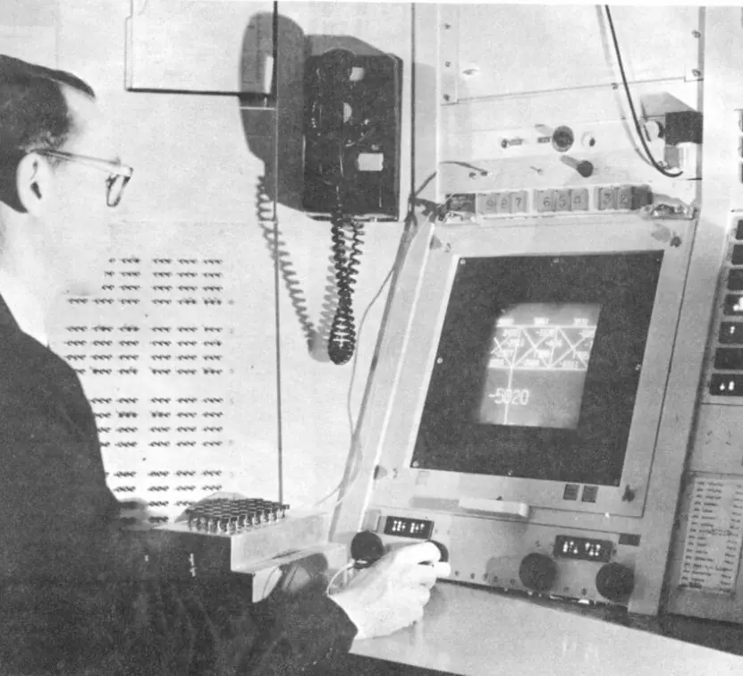
Scan conversion decides which pixels to light. Plate 2.1 pairs a historic photograph with a worked grid.
The photograph shows Ivan Sutherland at the TX-2 console in 1963 using Sketchpad, the first interactive drawing program, in which lines and circles were drawn on a display for the first time under program control.
The grid shows the pixels Bresenham's algorithm selects for the line from (5, 5) to (13, 10).


2.7.1 Eight reasons why Bresenham's algorithm is preferred for lines
- It uses only integers. The decision parameter changes by adding constants, so no floating-point numbers are needed. Integer addition is fast on every processor, from a phone to an embedded display controller. This was vital on early machines without floating-point hardware.
- It never rounds. DDA rounds a floating-point y at every step, and the small errors can add up on long lines. Bresenham's decision is exact for every pixel. The line it draws is always the closest set of pixels to the true line.
- It is faster than DDA. One comparison and one addition per pixel replace a multiplication and a rounding. For a long diagonal on a 1920-pixel screen the saving is visible. Graphics hardware therefore builds Bresenham-style logic into the chip.
- It works for every slope. By swapping the roles of x and y, and by changing the sign of the step, the same method handles all eight octants. A short wrapper chooses the right case. One routine can serve all lines in a drawing.
- It gives uniform brightness. Each column or row has exactly one pixel, so a line looks even without gaps or doubled pixels. Drawn on a plotter or LCD, the line appears straight. Quality is better than naive rounding.
- Its idea extends to circles and ellipses. The midpoint circle and ellipse algorithms use the same decision parameter and integer updates. Learning one algorithm prepares you for the others. A single idea draws most of the basic shapes.
- It is easy to implement and test. The whole algorithm is about ten lines of code. You can check it by hand with a table, as in the worked answers. Small code means fewer bugs.
- It is the basis of hardware rasterisers. GPUs draw millions of lines and triangle edges a second using incremental methods of the same type. A student who understands Bresenham understands why edge functions in GPUs are incremental. The method has lasted for sixty years.

Chapter summary
- Scan conversion picks pixels for primitives; step along the major axis and update an error term.
- DDA: steps = max(|Δx|, |Δy|), increments Δ/steps, round at each step; Bresenham uses p₀ = 2Δy − Δx and integer updates 2Δy or 2(Δy − Δx).
- Midpoint circle: p₀ = 1 − r, update by 2x + 1 (inside) or 2(x − y) + 1 (outside) with eight-way symmetry; midpoint ellipse uses two regions with four-way symmetry.
- Scan-line fill uses the odd–even rule; boundary and flood fill spread from a seed; antialiasing uses supersampling or coverage.
Practice
- Apply the DDA algorithm to (2, 3) to (7, 6). List the plotted pixels.
- State the decision parameters and update rules of Bresenham's algorithm for 0 < m < 1.
- Trace Bresenham from (1, 1) to (9, 5): give p₀ and the pixels.
- Why does the DDA need rounding but Bresenham does not?
- Why is only one octant computed for a circle, and how are the others obtained?
- Give p₀ for a midpoint circle of radius 8 and the first three octant pixels.
- Why are two regions needed for the ellipse algorithm?
- Explain the odd–even rule in scan-line filling.
- What is the difference between 4-connected and 8-connected boundary fill?
- Describe two antialiasing techniques.
Answers and worked solutions
1. Δx = 5, Δy = 3, steps = 5; x_inc = 1, y_inc = 0.6. Points: (2, 3), (3, 3.6→4), (4, 4.2→4), (5, 4.8→5), (6, 5.4→5), (7, 6.0→6): pixels (2,3), (3,4), (4,4), (5,5), (6,5), (7,6).
2. p₀ = 2Δy − Δx. If pₖ < 0: plot (x + 1, y), pₖ₊₁ = pₖ + 2Δy. Else plot (x + 1, y + 1), pₖ₊₁ = pₖ + 2Δy − 2Δx.
3. Δx = 8, Δy = 4; p₀ = 0. Constants: 2Δy = 8, 2(Δy − Δx) = −8. Sequence: p = 0 → y up (1,1)→(2,2), p = −8; p < 0 → (3,2), p = 0; → (4,3), p = −8; → (5,3), p = 0; → (6,4), p = −8; → (7,4), p = 0; → (8,5), p = −8; → (9,5). Pixels (1,1), (2,2), (3,2), (4,3), (5,3), (6,4), (7,4), (8,5), (9,5).
4. The DDA accumulates fractional coordinates, which must be rounded to pixels; Bresenham keeps only an integer error term that tells which integer pixel to choose.
5. The circle is symmetric about both axes and the line y = x, so each point (x, y) gives (±x, ±y) and (±y, ±x) (eight points).
6. p₀ = 1 − 8 = −7. First pixels: (0, 8); p < 0 → (1, 8), p = −7 + 3 = −4; p < 0 → (2, 8), p = −4 + 5 = 1; p ≥ 0 → (3, 7).
7. The slope changes from shallower than −1 to steeper than −1 around the quadrant, so stepping along x then along y keeps the step in the major direction.
8. Intersections of the scan line with the edges are sorted by x and paired; pixels between the 1st and 2nd, 3rd and 4th, … intersections are inside.
9. 4-connected fill spreads to up/down/left/right neighbours; 8-connected also uses the diagonals and can leak through diagonal gaps in a boundary.
10. Supersampling (render at higher resolution and average) and area/coverage sampling (intensity proportional to the covered fraction of the pixel).
Model answers: medium (5 marks) and long (10 marks) questions
Q1 (5 marks). Compare the DDA and Bresenham line-drawing algorithms.
Introduction. Both algorithms convert a line between two end points into the pixels of a raster display; they differ in how they decide the next pixel (sections 2.2, 2.3 and Figure 2.2).
- Method. DDA adds a fixed increment (1 and the slope) to the coordinates at every step and rounds the result. Bresenham keeps an integer decision parameter and chooses between two candidate pixels.
- Arithmetic. DDA uses floating-point addition and rounding; Bresenham uses integer addition and comparison only.
- Accuracy. Rounding errors can accumulate in DDA on long lines; Bresenham is exact for every pixel.
- Speed. Bresenham is faster and is easily put in hardware.
- Generality. DDA is simple to understand and to extend to any slope; Bresenham needs a case for each octant but one wrapper handles all of them.
| Point | DDA | Bresenham |
|---|---|---|
| Arithmetic | Floating point | Integer only |
| Rounding | Every step | None |
| Speed | Slower | Faster |
| Error | May accumulate | None |
| Ease | Very easy | Slightly harder |
Conclusion. DDA is good for teaching; Bresenham is the standard for real use.
Q2 (5 marks). Use Bresenham's algorithm to find the pixels of the line from (5, 5) to (13, 10).
Introduction. Here dx = 8 and dy = 5, so the slope is 0.625 (between 0 and 1) and we step x by one. The initial parameter is p0 = 2dy - dx = 10 - 8 = 2. If p < 0 plot (x + 1, y) and add 2dy = 10; otherwise plot (x + 1, y + 1) and add 2dy - 2dx = 10 - 16 = -6.
| k | p_k | Next pixel |
|---|---|---|
| start | p0 = 2*5 - 8 = 2 | (5, 5) |
| 0 | 2 | (6, 6) |
| 1 | -4 | (7, 6) |
| 2 | 6 | (8, 7) |
| 3 | 0 | (9, 8) |
| 4 | -6 | (10, 8) |
| 5 | 4 | (11, 9) |
| 6 | -2 | (12, 9) |
| 7 | 8 | (13, 10) |
Result. The pixels are (5, 5), (6, 6), (7, 6), (8, 7), (9, 8), (10, 8), (11, 9), (12, 9) and (13, 10): nine pixels, one per column, ending exactly at the end point (Plate 2.1).
The parameter ends at p = 8, and the last step used the "otherwise" branch because 8 is not negative.
Conclusion. Eight additions and eight comparisons produced the whole line without any division or rounding.
Q3 (10 marks). Explain the midpoint circle algorithm. Derive the decision parameter, state the steps and generate the first-octant pixels of a circle of radius 8 centred at the origin.
Introduction. A circle x^{2} + y^{2} = r^{2} is symmetric in eight ways, so only the octant from (0, r) to the line x = y needs to be computed; the other seven octants are reflections (Figure 2.1).
Circle function. f(x, y) = x^{2} + y^{2} - r^{2} is negative inside the circle, zero on it and positive outside. At each step x increases by 1 and the choice is between (x + 1, y) and (x + 1, y - 1).
Evaluate f at the midpoint (x + 1, y - 1/2); its value is the decision parameter p_k (Figure 2.2).
Derivation and steps. With the start (0, r) the first parameter is p0 = 1 - r. For each step: if p_k < 0 the midpoint is inside, so plot (x + 1, y) and p_k+1 = p_k + 2(x + 1) + 1; otherwise plot (x + 1, y - 1) and p_k+1 = p_k + 2(x + 1) + 1 - 2(y - 1).
Stop when x ≥ y, then plot the eight reflections of every point.
Worked example, r = 8. p0 = 1 - 8 = -7, first point (0, 8).
| k | p_k | Next (x, y) |
|---|---|---|
| 0 | -7 | (1, 8) |
| 1 | -4 | (2, 8) |
| 2 | 1 | (3, 7) |
| 3 | -6 | (4, 7) |
| 4 | 3 | (5, 6) |
| 5 | 2 | (6, 5) |
The step to (6, 5) has x > y, so the octant ends at (5, 6); (6, 5) is only the mirror image of (5, 6).
The octant pixels are (0, 8), (1, 8), (2, 8), (3, 7), (4, 7) and (5, 6): six calculated points give 8 x 6 = 48 plotted points before the duplicates on the axes and the diagonal are removed.
| Property | Value |
|---|---|
| Decision parameter start | 1 - r |
| Arithmetic | Integer only |
| Calculated points per circle | One octant |
| Reflections | Seven |
Conclusion. The midpoint circle algorithm uses the same idea as Bresenham's line algorithm: an incremental integer decision between two candidate pixels, made faster by symmetry.