Unit 1 · 6 teaching hours · 16 min read
Introduction
What the syllabus asks for 7
- Scarcity, choice and opportunity cost
- Economic systems
- Microeconomics and macroeconomics
- Goals and instruments of macroeconomics
- Demand, supply and market equilibrium
- Seeing the ideas: frontier, equilibrium and the people behind them
- Eight applications of economic thinking for a BCA student
Economics studies how individuals, firms and governments choose to use scarce resources to satisfy unlimited wants.
For a computing professional it explains pricing of software and cloud services, why markets for apps behave as they do, how inflation and interest rates affect a business, and how to compare costs and benefits.
All numbers in this book were recomputed by bca/tools/check_economics.py.
- Scarcity, choice, opportunity cost and the production possibility frontier.
- Microeconomics versus macroeconomics; positive versus normative economics.
- Goals and instruments of macroeconomic policy.
- Demand, supply and market equilibrium: the base for every later unit.
1.1 Scarcity, choice and opportunity cost
Wants are unlimited; resources (land, labour, capital, entrepreneurship) are limited. This scarcity forces choice, and every choice has an opportunity cost: the value of the best alternative given up.
A student who spends an evening on a freelance job (earning NPR 2,000) instead of studying bears an opportunity cost of the study time; a firm using its own building bears the rent it could have earned.
The three central questions of any economy: what to produce, how to produce it, and for whom.
Production possibility frontier (PPF): the maximum combinations of two goods an economy can produce with its resources and technology.
Suppose it can make 100 laptops or 400 tonnes of rice, or intermediate combinations such as 60 laptops and 280 tonnes. Points on the curve are efficient; points inside are wasteful (unemployment); points outside are unattainable now.
Moving along the curve shows opportunity cost (more laptops, less rice); economic growth shifts the curve outward.
If producing the first 10 extra laptops costs 20 tonnes of rice, the opportunity cost of a laptop is 2 tonnes; it usually rises as we specialise (bowed-out curve).
1.2 Economic systems
| System | Who decides | Example |
|---|---|---|
| Market (capitalist) | prices and private choices | USA (largely) |
| Command (socialist) | the state plans | former USSR |
| Mixed | markets plus government | Nepal, India, most countries |
Nepal's constitution describes a mixed economy with public, private and cooperative sectors.
1.3 Microeconomics and macroeconomics
| Microeconomics | Macroeconomics | |
|---|---|---|
| Studies | individual units: consumers, firms, single markets | the whole economy: total output, employment, price level |
| Key questions | How is the price of a product set? How much will a firm produce? | Why does inflation rise? What determines GDP growth and unemployment? |
| Tools | demand and supply, elasticity, cost curves, market structures | national income accounts, money, fiscal and monetary policy, trade |
| Variables | price of one good, output of one firm | GDP, inflation rate, unemployment |
They are linked: macro outcomes are the sum of micro decisions, but what is true for one (saving more is good for a family) can be false for all (if everyone saves, spending and income fall: the paradox of thrift: a fallacy of composition).
Positive economics describes what is (a testable statement: "a 10% price rise reduced sales by 15%"); normative economics states what ought to be (a value judgement: "the minimum wage should be raised").
1.4 Goals and instruments of macroeconomics
| Goal | Meaning | Measure |
|---|---|---|
| Economic growth | rising real output per person | growth rate of real GDP |
| Price stability | low and stable inflation | inflation rate (CPI) |
| Full employment | minimal involuntary unemployment | unemployment rate |
| Balance of payments equilibrium and stable exchange rate | sustainable external position | current account, reserves |
| Equitable distribution and poverty reduction | fair sharing of income | Gini coefficient, poverty rate |
| Instrument | Controlled by | Tools |
|---|---|---|
| Fiscal policy | government | taxes, public spending, borrowing (budget) |
| Monetary policy | central bank (Nepal Rastra Bank) | money supply, reserve ratios, policy interest rates |
| Trade and exchange-rate policy | government/central bank | tariffs, quotas, exchange-rate regime |
| Income and price policy / supply-side measures | government | minimum wages, price controls, investment incentives |
Goals can conflict: expansionary policy reduces unemployment but may raise inflation (the Phillips-curve trade-off).
1.5 Demand, supply and market equilibrium
Demand: the quantity buyers are willing and able to buy at each price. Law of demand: other things equal, quantity demanded falls as price rises (negative slope).
Determinants (shifting the curve): income, prices of related goods (substitutes, complements), tastes, population, expectations. A change in price causes movement along the curve; a change in any other determinant shifts it.
Supply: quantity sellers offer at each price; law of supply: quantity supplied rises with price. Shifters: input costs, technology, taxes and subsidies, number of sellers, expectations.
Equilibrium is the price at which quantity demanded equals quantity supplied; above it there is a surplus (price falls), below it a shortage (price rises).
Demand Q_d = 100 − 2P; supply Q_s = 20 + 3P. Equilibrium: 100 − 2P = 20 + 3P → 80 = 5P → P* = 16, Q* = 100 − 32 = 68 (check: 20 + 48 = 68). Price ceiling at P = 10: Q_d = 80, Q_s = 50 → shortage of 30 units (queues, black markets).
Demand increases to Q_d = 120 − 2P: 120 − 2P = 20 + 3P → P = 20, Q = 80: both rise. Tax of NPR 5 per unit on sellers: supply becomes Q_s = 20 + 3(P − 5) = 5 + 3P; 100 − 2P = 5 + 3P → P = 19, Q = 62.
Buyers pay 19 (up 3), sellers receive 19 − 5 = 14 (down 2); tax revenue = 5 × 62 = 310. The burden is shared (buyers 3/5 here), the more inelastic side bearing more (Unit 2).
Consumer and producer surplus: consumer surplus is the gap between what buyers would pay and what they do pay; producer surplus the gap between price received and minimum acceptable price.
Total surplus is largest at equilibrium; price controls and taxes create a deadweight loss.
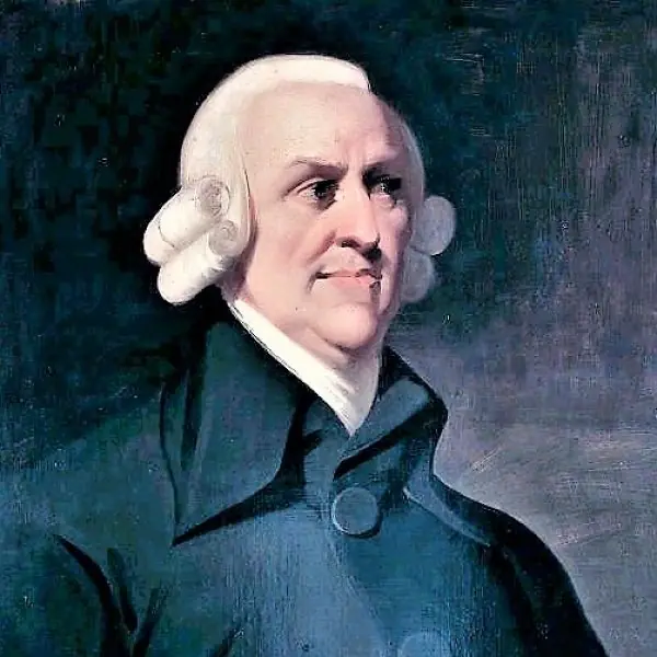
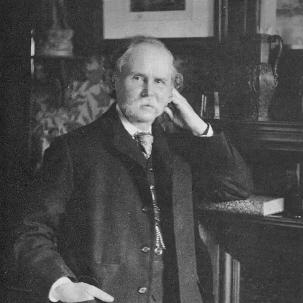
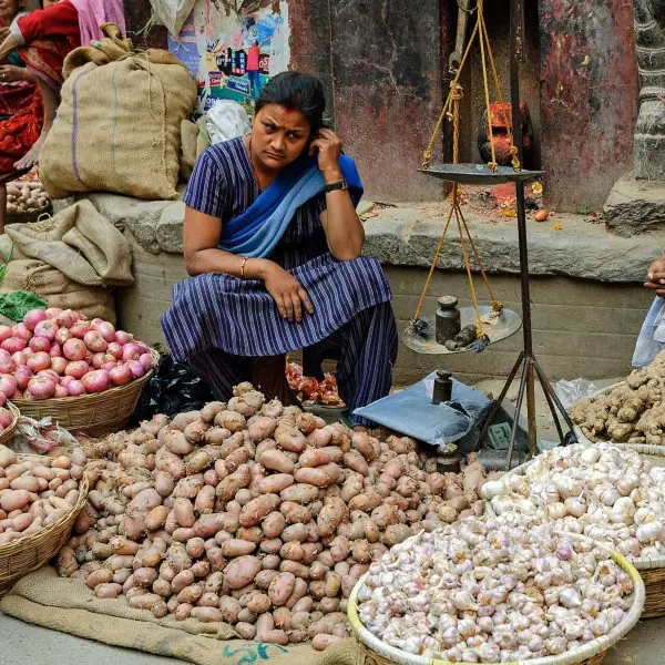
1.6 Seeing the ideas: frontier, equilibrium and the people behind them
The two graphs below are the working tools of the whole subject; the plate shows who built them and where they apply.


1.7 Eight applications of economic thinking for a BCA student
- Opportunity cost in daily choices. Every hour has a best alternative use, so a student who spends a Saturday on a freelance website job gives up that day of revision. Counting the forgone alternative, and not only the money paid, leads to wiser choices. A Kathmandu start-up deciding between building its own server room and renting cloud space makes the same comparison.
- Pricing a product or service. Demand and supply tell a software firm how many subscriptions it can sell at each price. If the price is set above equilibrium, subscriptions pile up unsold, and if it is set too low, the servers are overloaded. Nepali apps such as ride-hailing and food delivery change prices by the hour for exactly this reason.
- Understanding shortages and queues. A price ceiling holds the price below equilibrium, so buyers want more than sellers will supply. The result is queues and black markets, as seen in fuel and cooking-gas shortages in Nepal. Knowing the cause helps a student judge whether a control will really help consumers.
- Judging taxes and subsidies. A tax on sellers raises the price to buyers and lowers the price received by sellers, so both share the burden. The Value Added Tax on a mobile recharge card or a laptop works in this way. A student can compute who pays how much, as in the NPR 5 example above.
- Reading macroeconomic news. Terms such as GDP growth, inflation and the budget deficit appear daily in news about the Nepal Rastra Bank and the Ministry of Finance. The five macroeconomic goals give a checklist for judging any policy. A citizen who knows them can separate a real improvement from a slogan.
- Planning the economy's use of resources. The production possibility frontier shows that more roads mean fewer schools unless the economy grows. Nepal faces such choices every year when the budget is divided between hydropower, education and health. The frontier turns this vague argument into a clear trade-off.
- Business and career decisions. A graduate choosing between a job in Kathmandu and one abroad weighs wages, living costs and migration expenses. This is cost-benefit thinking, the same tool a bank uses to approve a loan. Economic reasoning makes the comparison honest and complete.
- Designing and valuing technology. Digital payments, such as Fonepay, eSewa and ConnectIPS, change transaction costs and shift the supply of banking services. Free software and open data show how a product with zero extra cost per user is priced. The economics of such goods explains why platforms grow so fast.
Formula and fact sheet
- Opportunity cost = value of the best forgone alternative. PPF: efficient on the curve, growth shifts it out.
- Macro goals: growth, price stability, full employment, external balance, equity. Instruments: fiscal, monetary, trade/exchange rate.
- Equilibrium: Q_d = Q_s; shortage if price below, surplus if above.
- Movement along vs shift of a curve.
Chapter summary
- Scarcity forces choice, and each choice costs its best alternative; the PPF illustrates trade-offs and growth.
- Micro studies individual markets and decision-makers; macro studies aggregates; policy pursues several goals with fiscal, monetary and trade instruments.
- Demand and supply determine price and quantity; shifts, controls and taxes can be analysed with equations.
Practice
- Define scarcity and opportunity cost; give an example from student life.
- Distinguish micro and macroeconomics; positive and normative statements.
- List the macroeconomic goals and the main instruments.
- Q_d = 200 − 4P, Q_s = 50 + 2P. Find equilibrium; find the shortage or surplus at P = 20.
- Explain the difference between a movement along and a shift of the demand curve.
- What happens to price and quantity if supply increases (all else equal)?
- Explain the PPF and what a point inside it means.
Answers and worked solutions
1. Scarcity: limited resources against unlimited wants. Opportunity cost: the best alternative forgone; e.g. an evening at a part-time job instead of studying has the study time as its cost.
2. Micro: single markets and agents; macro: the whole economy. Positive: factual and testable; normative: involves values ("should").
3. Goals: growth, price stability, full employment, balance of payments, equity. Instruments: fiscal, monetary, trade/exchange-rate, income and supply-side policies.
4. 200 − 4P = 50 + 2P → 150 = 6P → P = 25, Q = 100. At P = 20: Q_d = 120, Q_s = 90 → shortage of 30.
5. A price change moves us along the same curve; a change in income, tastes, related prices or expectations shifts the whole curve.
6. Supply shifts right: equilibrium price falls, quantity rises.
7. The PPF shows the maximum outputs attainable; a point inside means resources are unemployed or misused (inefficiency); outside is unattainable with present resources.
Model answers: medium (5 marks) and long (10 marks) questions
Q1 (5 marks). Explain scarcity, choice and opportunity cost. Use a production possibility frontier to show them.
Introduction. Human wants are unlimited, but land, labour, capital and entrepreneurship are limited. This gap is called scarcity, and it forces every person and every nation to choose.
Key ideas.
- Scarcity: resources are not enough to satisfy all wants, so even a rich country cannot produce everything.
- Choice: the economy must decide what to produce, how to produce it, and for whom.
- Opportunity cost: the value of the best alternative given up. A student who works for NPR 2,000 instead of studying pays the cost of the study time.
Diagram (Figure 1.1). The frontier joins the largest combinations of laptops and rice the economy can make. For the example, A is 400 tonnes of rice and no laptops, B is 60 laptops and 280 tonnes, and C is 100 laptops and no rice.
Moving from A to B gives 60 laptops at the cost of 120 tonnes of rice, so a laptop costs 2 tonnes here. The curve bows outward because the cost rises as resources are moved to a job they suit less well.
A point inside the curve, such as U, means unemployment; a point outside, such as X, cannot be reached until growth shifts the curve outward.
Conclusion. The frontier is a picture of scarcity (the limit), choice (the position on it) and opportunity cost (its slope).
Q2 (5 marks). Distinguish between microeconomics and macroeconomics, and between positive and normative economics.
Introduction. Economics studies how society uses scarce resources. It is studied at two levels and with two kinds of statement.
| Point | Microeconomics | Macroeconomics |
|---|---|---|
| Unit of study | one consumer, firm or market | the whole economy |
| Main question | how is the price of rice or a phone plan set? | why does inflation rise, what decides GDP and jobs? |
| Tools | demand, supply, elasticity, cost curves | national income, money, fiscal and monetary policy |
| Variables | price and output of one good | GDP, price level, unemployment |
| Example | why a vegetable seller at Asan lowers the price in the evening | why Nepal's growth slowed in a year |
The two levels are linked. Macro results are the sum of micro decisions, but a truth for one person may be false for all. If one family saves more it becomes richer; if every family saves more, spending and income fall (the paradox of thrift).
Positive and normative. A positive statement says what is and can be tested: "a 10% price rise reduced sales by 15%". A normative statement says what ought to be, a value judgement: "the minimum wage should be raised".
Conclusion. Micro looks at the trees and macro at the forest; positive economics gives the facts and normative economics gives the opinion.
Q3 (10 marks). Explain the laws of demand and supply and the determination of equilibrium price. Using Q_d = 100 − 2P and Q_s = 20 + 3P, show the effect of a price ceiling, a rise in demand and a tax of NPR 5 per unit.
Introduction. In a market economy the price of a good is set by the interaction of buyers and sellers. Demand is the quantity buyers are willing and able to buy at each price; supply is the quantity sellers offer at each price (Figure 1.2).
Laws. (1) Law of demand: other things equal, a higher price lowers the quantity demanded, so the demand curve slopes down.
(2) Law of supply: other things equal, a higher price raises the quantity supplied, so the supply curve slopes up. A change in price moves the point along the curve.
A change in income, tastes, the price of related goods, population or expectations shifts the demand curve; a change in input costs, technology, taxes or the number of sellers shifts the supply curve.
Equilibrium. At the price where Q_d = Q_s the market clears. Above it there is a surplus and the price falls; below it there is a shortage and the price rises.
Numerical illustration.
- Equilibrium: 100 − 2P = 20 + 3P gives 80 = 5P, so P* = 16 and Q* = 68 (check: 20 + 48 = 68). Consumer surplus is the triangle under the demand curve above the price: ½ × (50 − 16) × 68 = 1,156.
- Price ceiling at 10: Q_d = 80 and Q_s = 50, so there is a shortage of 30 units. Queues, rationing and black markets follow.
- Rise in demand to Q_d = 120 − 2P: 120 − 2P = 20 + 3P gives P = 20 and Q = 80. Both price and quantity rise.
- Tax of NPR 5 on sellers: supply becomes Q_s = 5 + 3P, so 100 − 2P = 5 + 3P gives P = 19 and Q = 62. Buyers pay 3 more, sellers keep 14 (2 less), the government collects 5 × 62 = 310, and the deadweight loss is ½ × 5 × (68 − 62) = 15.
Comparison of the three interventions.
| Event | New price | New quantity | Effect |
|---|---|---|---|
| Starting equilibrium | 16 | 68 | market clears |
| Ceiling at 10 | 10 | 50 sold | shortage of 30 |
| Demand rises | 20 | 80 | price and quantity both up |
| Tax of 5 | 19 (buyers) | 62 | burden shared 3 : 2, DWL 15 |
Conclusion. Prices ration scarce goods and send signals to buyers and sellers. Controls and taxes change the outcome and, away from equilibrium, waste some of the gains from trade.