Unit 7 · 7 teaching hours · 23 min read
Data Analysis and Visualisation: NumPy, Pandas, Matplotlib
What the syllabus asks for 4
- NumPy
- Pandas
- Matplotlib
- Seeing the ideas: data made visible
Python became the language of data because of three libraries: NumPy (fast numerical arrays), Pandas (tables of data with labels) and Matplotlib (charts). Together they replace spreadsheet gymnastics with a few clear lines of code.
- NumPy arrays: creation, indexing, slicing, vectorised operations, broadcasting, statistics.
- Pandas Series and DataFrame: loading data, selecting, filtering, grouping, handling missing values.
- Matplotlib: line, bar, histogram and pie charts saved to files.
The libraries are installed with pip install numpy pandas matplotlib. The outputs below come from NumPy 2.5, Pandas 3.1 and Matplotlib 3.11 on Python 3.12; the layout of printed tables can differ slightly in other versions.
7.1 NumPy
A NumPy ndarray holds items of one type in a compact block of memory and applies operations to the whole array at once (vectorisation), which is typically tens to hundreds of times faster than a Python loop.
import numpy as np
a = np.array([3, 1, 4, 1, 5, 9, 2, 6])
print(a, a.dtype, a.shape, a.ndim, a.size)
print(np.arange(0, 10, 2), np.linspace(0, 1, 5), np.zeros((2, 3)), np.eye(2), sep="\n")
m = np.arange(12).reshape(3, 4)
print(m, m.T.shape, m[1, 2], m[:, 1], m[1:, ::2], sep="\n")
[3 1 4 1 5 9 2 6] int64 (8,) 1 8
[0 2 4 6 8]
[0.   0.25 0.5  0.75 1.  ]
[[0. 0. 0.]
 [0. 0. 0.]]
[[1. 0.]
 [0. 1.]]
[[ 0  1  2  3]
 [ 4  5  6  7]
 [ 8  9 10 11]]
(4, 3)
6
[1 5 9]
[[ 4  6]
 [ 8 10]]
Vectorised operations and broadcasting
import numpy as np
x = np.array([1.0, 2.0, 3.0, 4.0])
print(x * 2, x ** 2, x + np.array([10, 20, 30, 40]), np.sqrt(x))
m = np.arange(6).reshape(2, 3)
print(m + np.array([100, 200, 300]))
print(m * np.array([[1], [10]]))
print(x > 2, x[x > 2], np.where(x > 2, "big", "small"))
[2. 4. 6. 8.] [ 1.  4.  9. 16.] [11. 22. 33. 44.] [1.         1.41421356 1.73205081 2.        ]
[[100 201 302]
 [103 204 305]]
[[ 0  1  2]
 [30 40 50]]
[False False  True  True] [3. 4.] ['small' 'small' 'big' 'big']
Broadcasting stretches the smaller array to the shape of the larger when their shapes are compatible (equal, or 1, in each dimension from the right): a row is added to every row of the matrix; a column multiplies every column.
Statistics and linear algebra
import numpy as np
marks = np.array([[72, 65, 80], [90, 85, 95], [55, 60, 58], [78, 82, 70]])
print(marks.mean(), marks.mean(axis=0), marks.max(axis=1), marks.sum(axis=0))
print(np.median(marks), round(marks.std(), 3), marks.argmax(), np.sort(marks[:, 0]))
A = np.array([[2.0, 1.0], [1.0, 3.0]])
b = np.array([5.0, 10.0])
x = np.linalg.solve(A, b)
print(x, A @ x, np.linalg.det(A), np.linalg.inv(A).round(3))
rng = np.random.default_rng(42)
print(rng.integers(1, 7, size=8), rng.normal(0, 1, 3).round(3))
74.16666666666667 [73.75 73.   75.75] [80 95 60 82] [295 292 303]
75.0 12.409 5 [55 72 78 90]
[1. 3.] [ 5. 10.] 5.000000000000001 [[ 0.6 -0.2]
 [-0.2  0.4]]
[1 5 4 3 3 6 1 5] [-1.951 -1.302  0.128]
axis=0 works down the columns, axis=1 along the rows; @ is matrix multiplication; np.linalg solves linear systems (the Numerical Methods book of this semester does it by hand). Seeding the random generator makes results reproducible.
7.2 Pandas
A Series is a labelled one-dimensional array; a DataFrame is a table of Series sharing an index, much like a spreadsheet or SQL table.
import pandas as pd
s = pd.Series([88, 92, 79], index=["Ram", "Sita", "Hari"], name="marks")
print(s, s["Sita"], s.mean(), s[s > 80].index.tolist(), sep="\n")
df = pd.DataFrame({"name": ["Ram", "Sita", "Hari", "Gita"],
                   "dept": ["BCA", "BCA", "BIT", "BIT"],
                   "marks": [78, 91, 64, 85]})
print(df)
print(df.shape, list(df.columns), df["marks"].dtype)
print(df.describe().round(2))
Ram     88
Sita    92
Hari    79
Name: marks, dtype: int64
92
86.33333333333333
['Ram', 'Sita']
   name dept  marks
0   Ram  BCA     78
1  Sita  BCA     91
2  Hari  BIT     64
3  Gita  BIT     85
(4, 3) ['name', 'dept', 'marks'] int64
       marks
count   4.00
mean   79.50
std    11.62
min    64.00
25%    74.50
50%    81.50
75%    86.50
max    91.00
Loading data
pd.read_csv("file.csv") loads a CSV file into a DataFrame (read_excel, read_json, read_sql do likewise). Here the file content is supplied from a string so that the example is self-contained; it contains a missing value.
import io
import pandas as pd
csv_text = """roll,name,dept,maths,physics
1,Ram,BCA,78,70
2,Sita,BCA,91,
3,Hari,BIT,64,58
4,Gita,BIT,85,90
5,Bikash,BCA,55,62
"""
df = pd.read_csv(io.StringIO(csv_text))
print(df)
print(df.isna().sum().to_dict())
df["physics"] = df["physics"].fillna(df["physics"].mean())
df["total"] = df["maths"] + df["physics"]
print(df[["name", "total"]])
   roll    name dept  maths  physics
0     1     Ram  BCA     78     70.0
1     2    Sita  BCA     91      NaN
2     3    Hari  BIT     64     58.0
3     4    Gita  BIT     85     90.0
4     5  Bikash  BCA     55     62.0
{'roll': 0, 'name': 0, 'dept': 0, 'maths': 0, 'physics': 1}
     name  total
0     Ram  148.0
1    Sita  161.0
2    Hari  122.0
3    Gita  175.0
4  Bikash  117.0
Selecting, filtering, sorting, grouping
import io
import pandas as pd
df = pd.read_csv(io.StringIO("""name,dept,maths,physics
Ram,BCA,78,70
Sita,BCA,91,80
Hari,BIT,64,58
Gita,BIT,85,90
Bikash,BCA,55,62
"""))
print(df[df["maths"] > 70])
print(df.loc[df["dept"] == "BCA", ["name", "maths"]])
print(df.sort_values("maths", ascending=False).head(3)["name"].tolist())
print(df.iloc[1:3, 0:2])
g = df.groupby("dept")[["maths", "physics"]].mean().round(1)
print(g)
print(df.groupby("dept").agg(students=("name", "count"), best=("maths", "max")))
   name dept  maths  physics
0   Ram  BCA     78       70
1  Sita  BCA     91       80
3  Gita  BIT     85       90
     name  maths
0     Ram     78
1    Sita     91
4  Bikash     55
['Sita', 'Gita', 'Ram']
   name dept
1  Sita  BCA
2  Hari  BIT
      maths  physics
dept
BCA    74.7     70.7
BIT    74.5     74.0
      students  best
dept
BCA          3    91
BIT          2    85
loc selects by label and conditions; iloc by integer position. groupby splits the rows, applies a function (mean, count, max) to each group and combines the results, the same idea as SQL GROUP BY.
Other staples: merge (join two tables), pivot_table, value_counts, apply, drop_duplicates, to_csv.
import pandas as pd
a = pd.DataFrame({"dept": ["BCA", "BIT"], "head": ["Dr. Shah", "Dr. Rai"]})
b = pd.DataFrame({"name": ["Ram", "Hari", "Zed"], "dept": ["BCA", "BIT", "BBA"]})
print(b.merge(a, on="dept", how="left"))
print(pd.Series(["a", "b", "a", "c", "a"]).value_counts().to_dict())
   name dept      head
0   Ram  BCA  Dr. Shah
1  Hari  BIT   Dr. Rai
2   Zed  BBA       NaN
{'a': 3, 'b': 1, 'c': 1}
7.3 Matplotlib
Matplotlib draws charts. In a script you build a figure and either plt.show() it or plt.savefig("name.png"). The programs below save files (a non-interactive backend) and print what was produced.
import matplotlib
matplotlib.use("Agg")
import matplotlib.pyplot as plt
import numpy as np, os
x = np.linspace(0, 2 * np.pi, 100)
fig, ax = plt.subplots(figsize=(6, 3))
ax.plot(x, np.sin(x), label="sin x", color="tab:blue")
ax.plot(x, np.cos(x), "--", label="cos x", color="tab:red")
ax.set(title="Sine and cosine", xlabel="x (radians)", ylabel="value")
ax.legend(); ax.grid(True)
fig.tight_layout()
fig.savefig("trig.png", dpi=100)
print(os.path.exists("trig.png"), fig.get_size_inches(), len(ax.lines))
True [6. 3.] 2
import matplotlib
matplotlib.use("Agg")
import matplotlib.pyplot as plt
import numpy as np
fig, axes = plt.subplots(1, 3, figsize=(10, 3))
subjects, avg = ["OS", "NM", "SE", "Py", "WT"], [68, 61, 72, 80, 75]
axes[0].bar(subjects, avg, color="tab:green"); axes[0].set_title("Bar chart")
rng = np.random.default_rng(1)
data = rng.normal(60, 12, 200)
axes[1].hist(data, bins=10, edgecolor="black"); axes[1].set_title("Histogram")
axes[2].pie([40, 30, 20, 10], labels=["A", "B", "C", "D"], autopct="%1.0f%%"); axes[2].set_title("Pie chart")
fig.tight_layout(); fig.savefig("charts.png")
counts, edges = np.histogram(data, bins=10)
print(len(axes), counts.sum(), round(data.mean(), 1), round(data.std(), 1))
3 200 59.1 11.1
| Chart | Use | Call |
|---|---|---|
| Line | trends over an ordered axis | plot |
| Bar | compare categories | bar, barh |
| Histogram | distribution of one variable | hist |
| Scatter | relationship between two variables | scatter |
| Pie | parts of a whole (few slices only) | pie |
Good charts have a title, labelled axes with units, a legend when several series appear, and no unnecessary decoration. Pandas can draw directly: df.plot(kind="bar").
7.4 Seeing the ideas: data made visible
Long before NumPy and Pandas, people turned numbers into pictures so that a pattern could be seen at once.
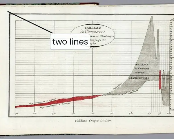
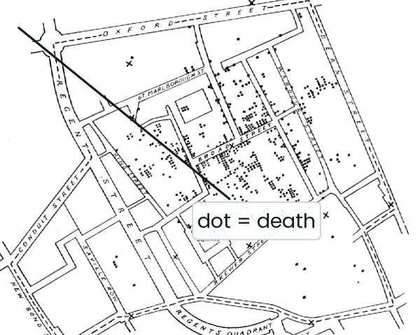
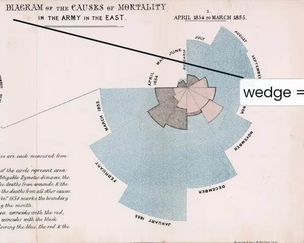
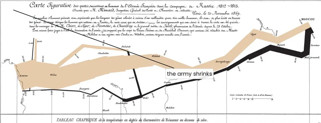
The three historical charts below were each drawn by hand, and each one matches a chart type you can now make in a few lines of Matplotlib.
After them, the figures show how broadcasting and axis work in NumPy, how groupby splits and combines a table, what the parts of a Matplotlib figure are, and what a real histogram looks like.


7.4.1 Eight applications of Python data analysis
- Examination and school results. A board or a college holds thousands of marks in a table. With Pandas,
groupby("district")["pass"].mean()gives the pass rate of every district in one line, and a bar chart shows the weak districts. Tribhuvan University and school education management systems (EMIS) use this kind of summary every year to plan teacher support. - Banking and digital payments. Wallets and bank transfers such as ConnectIPS and Fonepay produce a record for every payment. Pandas can total the payments per hour and Matplotlib can draw the daily curve, so the busiest hours are seen at once. Values that are far from the rest (outliers) can be flagged for a fraud check.
- Stock market (NEPSE). A table of daily closing prices becomes a line chart in two lines of code. A moving average, such as
rolling(20).mean(), smooths the noise and shows the trend. This helps a student of finance to study a company's price history before writing a report. - Weather and floods. The Department of Hydrology and Meteorology records rainfall and river levels every day. NumPy handles the long arrays of readings, and a line chart of the monsoon months shows when a river is rising. Such charts support early warning to villages along the river.
- Census and planning. A census gives a table of population, households and literacy for each district.
mergejoins it with a second table (for example school counts) andsort_valuesfinds the districts with the lowest services. Plans for roads, schools and clinics can then be based on numbers instead of guesses. - Public health. A weekly count of dengue or diarrhoea cases is a time series. Plotting it shows an outbreak starting, as John Snow's map did for cholera (Plate 7.1). Grouping the cases by ward then shows where to send the health team first.
- Electricity and energy. The Nepal Electricity Authority needs the load of the grid every hour. A NumPy array of 24 values per day can be averaged over a month with
mean(axis=0), and the peak hour is found withargmax. The result guides when to start extra generation or to ask users to save power in the evening. - Tourism and small business. Monthly arrivals of tourists, or the daily sales of a shop in Pokhara, fit in one DataFrame. A bar chart by month shows the season, and
groupbyon product shows what sells. The owner can plan stock, staff and prices from the pattern.
Formula and fact sheet
np.array,arange,linspace,zeros,reshape; vectorised arithmetic; boolean masks;axis=0columns,axis=1rows.- Broadcasting: shapes compatible from the right (equal or 1).
pd.Series,pd.DataFrame,read_csv,loc(labels),iloc(positions),groupby().agg(),merge,fillna,isna.plt.subplots,plot/bar/hist/pie,savefig.
Chapter summary
- NumPy arrays give fast, vectorised numerical work with broadcasting and built-in statistics and linear algebra.
- Pandas turns CSV-style data into DataFrames that can be cleaned, filtered, grouped and merged in a few expressions.
- Matplotlib communicates the results as charts.
Practice
- Create a NumPy array of the squares of 1 to 10 and print those greater than 30.
- Explain broadcasting with an example of adding a vector to a matrix.
- Compute the mean of each column of a 3 × 3 array.
- Given a DataFrame of student marks, show how to find the students with more than 70 in maths.
- Group a DataFrame by department and report the mean marks.
- How would you handle missing values in a column?
- Plot y = x² for x from −3 to 3 and save the figure.
Answers and worked solutions
1.
import numpy as np
sq = np.arange(1, 11) ** 2
print(sq, sq[sq > 30])
[ 1 4 9 16 25 36 49 64 81 100] [ 36 49 64 81 100]
2.
import numpy as np
print(np.ones((2, 3)) + np.array([1, 2, 3]))
[[2. 3. 4.]
 [2. 3. 4.]]
The vector of shape (3,) is stretched across both rows of the (2, 3) array. 3.
import numpy as np
a = np.arange(9).reshape(3, 3)
print(a.mean(axis=0))
[3. 4. 5.]
4.
import pandas as pd
df = pd.DataFrame({"name": ["A", "B", "C"], "maths": [65, 82, 74]})
print(df[df["maths"] > 70]["name"].tolist())
['B', 'C']
5.
import pandas as pd
df = pd.DataFrame({"dept": ["BCA", "BIT", "BCA"], "marks": [70, 60, 90]})
print(df.groupby("dept")["marks"].mean().to_dict())
{'BCA': 80.0, 'BIT': 60.0}
6. Count them with df.isna().sum(); then either drop (dropna()), fill with a constant or statistic (fillna(df["col"].mean())), or interpolate, depending on how much is missing and why.
7.
import matplotlib
matplotlib.use("Agg")
import matplotlib.pyplot as plt
import numpy as np
x = np.linspace(-3, 3, 61)
plt.plot(x, x ** 2)
plt.title("y = x squared")
plt.savefig("parabola.png")
print(len(x), x.min(), (x ** 2).min())
61 -3.0 0.0
Model answers (5 and 10 marks)
Q1. What is a NumPy array? Explain vectorisation, broadcasting and the axis argument with a program. (5 marks)
Introduction. A NumPy ndarray is a fixed-size grid of items that all have the same type, stored together in one block of memory.
Because the type is fixed and the items sit side by side, NumPy can run loops in fast compiled code instead of in the Python interpreter. This makes array work many times faster than the same work on a list, and it needs much less code.
Main points.
- Creation and shape. Arrays are made with
np.array,arange,linspace,zerosandeye. The attributesshape,ndim,sizeanddtypedescribe the array, andreshapechanges the shape without changing the data. - Vectorisation. An operation such as
x * 2ornp.sqrt(x)is applied to every element at once, so noforloop is written. A comparison such asx > 2gives a Boolean array that can be used as a mask,x[x > 2]. - Broadcasting. When two arrays have different shapes, NumPy stretches the smaller one so the shapes match, provided that, comparing from the right, each pair of sizes is equal or one of them is 1 (Fig. 7.2).
- The axis argument.
axis=0collapses the rows and gives one result per column;axis=1collapses the columns and gives one result per row (Fig. 7.3).
import numpy as np
marks = np.array([[72, 65, 80], [90, 85, 95], [55, 60, 58], [78, 82, 70]])
print(marks.shape, marks.dtype)
print(marks.mean(axis=0).round(2))          # per subject
print(marks.max(axis=1))                    # per student
print(marks + np.array([5, 0, 0]))          # broadcasting: +5 to the first subject
print(marks[marks > 90])                    # Boolean mask
(4, 3) int64
[73.75 73.   75.75]
[80 95 60 82]
[[77 65 80]
 [95 85 95]
 [60 60 58]
 [83 82 70]]
[95]
Example. A teacher can add five grace marks to one subject for all students with the single expression marks + [5, 0, 0], and find the best mark of every student with marks.max(axis=1), without writing any loop.
Conclusion. NumPy arrays give compact storage, loop-free vectorised arithmetic, flexible broadcasting and one-line statistics, which is why Pandas and Matplotlib are built on top of them.
Q2. Distinguish between a Pandas Series and a DataFrame. Explain how rows are selected, filtered and grouped, with a program. (5 marks)
Introduction. Pandas is the library for working with tables of data that have labels.
Its two main objects are the Series, a labelled one-dimensional array, and the DataFrame, a two-dimensional table in which every column is a Series and all columns share one row index.
A DataFrame is much like a spreadsheet sheet or an SQL table, but it is controlled from code and can hold millions of rows.
Main points.
- Series versus DataFrame. A Series has one column of values and an index (for example marks labelled by student name). A DataFrame has many named columns that may have different types (text, integers, decimals).
- Loading.
pd.read_csv("file.csv")reads a table from a file, andhead(),info()anddescribe()give a quick look at its contents and statistics. - Selecting.
df["maths"]gives a column;df.loc[rows, columns]selects by label;df.iloc[i:j, k:l]selects by position. - Filtering. A Boolean condition such as
df["maths"] > 70keeps only the rows where it is true; conditions can be combined with&and|. - Grouping.
groupby("dept")splits the rows by a column, applies a function such asmeanorcountto every group and combines the results into a new table (Fig. 7.1).
import io
import pandas as pd
df = pd.read_csv(io.StringIO("""name,dept,maths
Ram,BCA,78
Sita,BCA,91
Hari,BIT,64
Gita,BIT,85
Bikash,BCA,55
"""))
print(type(df["maths"]).__name__, df.shape)
print(df[df["maths"] > 70]["name"].tolist())
print(df.loc[df["dept"] == "BCA", "maths"].max())
print(df.groupby("dept")["maths"].agg(["count", "mean"]).round(2))
Series (5, 3)
['Ram', 'Sita', 'Gita']
91
      count   mean
dept
BCA       3  74.67
BIT       2  74.50
Example. A college office can list all students above 70 in maths and the average of each department with three short expressions, and then send the result to a chart.
Conclusion. A Series holds one labelled column and a DataFrame holds a whole table; selection, Boolean filtering and groupby are the three operations that answer most questions asked of a table.
Q3. Explain data visualisation with Matplotlib. Describe the parts of a figure, the common chart types and how to choose between them, with a program. (10 marks)
Introduction. Data visualisation means turning numbers into a picture so that a pattern, a trend or an unusual value can be seen quickly.
People did this long before computers: Playfair's trade chart, Snow's cholera map and Nightingale's mortality diagram (Plate 7.1) each changed a decision.
Matplotlib is the standard Python library for drawing such charts, and it can save them as image files (PNG, PDF, SVG) for reports and web pages.
Parts of a figure (Fig. 7.4). The Figure is the whole canvas. An Axes is one plot area; a figure can hold several, created with plt.subplots(rows, columns).
Each Axes has an x-axis and a y-axis (ticks and labels), a title, an optional legend, a grid, and the artists that are drawn, such as lines, bars and text.
The recommended style is the object-oriented one: fig, ax = plt.subplots() and then ax.plot(...), ax.set(...).
Common chart types and their use.
- Line chart (
plot) for a trend over an ordered axis such as time, for example the daily NEPSE closing price. - Bar chart (
bar,barh) to compare a few categories, for example the average marks of five subjects. - Histogram (
hist) to show how the values of one variable are spread (Fig. 7.5). The bins are equal-width ranges and the height is the count in each. - Scatter plot (
scatter) to see whether two variables are related, for example study hours and marks. - Pie chart (
pie) for parts of a whole, only when there are very few slices.
import matplotlib
matplotlib.use("Agg")
import matplotlib.pyplot as plt
import numpy as np
rng = np.random.default_rng(1)
hours = rng.uniform(1, 8, 30)
marks = 40 + 6 * hours + rng.normal(0, 5, 30)
fig, (a1, a2) = plt.subplots(1, 2, figsize=(8, 3))
a1.scatter(hours, marks, color="tab:blue"); a1.set(title="Study hours vs marks", xlabel="hours per day", ylabel="marks")
a2.hist(marks, bins=8, edgecolor="black"); a2.set(title="Marks", xlabel="marks", ylabel="students")
fig.tight_layout(); fig.savefig("study.png", dpi=100)
r = np.corrcoef(hours, marks)[0, 1]
print(len(fig.axes), round(float(r), 2))
2 0.94
Choosing a chart.
| Question | Chart | Call |
|---|---|---|
| How does a value change over time? | Line | plot |
| Which category is larger? | Bar | bar |
| How are the values spread? | Histogram | hist |
| Are two variables related? | Scatter | scatter |
| What share does each part have? | Pie (few slices) | pie |
Good practice. Give every chart a title, label both axes with units, add a legend when there is more than one series, start a bar chart at zero, and avoid decoration that carries no data.
Minard's chart (Plate 7.2) is admired because every visual element carries information.
Conclusion. Matplotlib turns a table into a chart with a few lines; by understanding the Figure/Axes structure and choosing the chart type that matches the question, a student can communicate results clearly in a project report.
Q4. How are missing values handled in Pandas? Write a program and discuss when each method is suitable. (5 marks)
Introduction. Real data are rarely complete: a student may have been absent from an exam, or a sensor may have failed on one day. Pandas marks such gaps as NaN (not a number).
Most statistics skip NaN automatically, but if the gaps are not handled, counts, plots and models can be misleading, so cleaning is the first step of any analysis.
Main points.
- Detect.
df.isna()gives True where a value is missing, anddf.isna().sum()counts the gaps in each column (Fig. 7.6). - Drop.
dropna()removes rows (or columns) that contain gaps. It is simple and honest, but it throws away the other values in those rows, so it suits data where only a few rows are affected. - Fill with a constant or a statistic.
fillna(0)orfillna(s.mean())keeps every row. The mean or median keeps the average roughly unchanged but hides the fact that the value was missing, so use the median if there are outliers. - Fill from neighbours.
ffill()copies the previous value andinterpolate()draws a line between the neighbours; this suits a time series such as daily rainfall (a gap at the very end is simply copied from the last known value).
import pandas as pd, numpy as np
s = pd.Series([78, np.nan, 64, 85, np.nan], name="marks")
print(int(s.isna().sum()), round(float(s.mean()), 2))
print(s.dropna().tolist())
print(s.fillna(s.mean()).round(2).tolist())
print(s.interpolate().tolist())
2 75.67
[78.0, 64.0, 85.0]
[78.0, 75.67, 64.0, 85.0, 75.67]
[78.0, 71.0, 64.0, 85.0, 85.0]
Example. If two marks out of five are missing, the mean of the three known marks is 75.67. Dropping the rows leaves three students; filling with the mean keeps five students but gives two of them an invented mark.
Conclusion. First count the missing values, then choose to drop, fill with a statistic or interpolate according to how many are missing and why, and always record which choice was made.