Unit 8 · 2 teaching hours · 28 min read
Managing Software Projects
What the syllabus asks for 7
- Management activities and the need for management
- Project planning
- Estimating cost and effort
- Project scheduling
- Risk management
- Managing people
- Project management in pictures: estimates, networks and earned value
A project is late one day at a time. Software project management makes sure that a system is delivered on time and within budget while meeting requirements.
The syllabus gives this unit only two hours, but it is the unit of numbers: cost estimates, schedules, progress measurement and risk. Every figure below was recomputed in Python (bca/tools/check_se.py).
- Management activities and why software projects are hard to manage.
- Project planning and cost estimation: COCOMO (basic and intermediate) and function points.
- Project scheduling: the critical path method (CPM), PERT, and earned value management.
- Risk management and managing people.
8.1 Management activities and the need for management
Software is intangible (progress is invisible), each project is one-off, processes vary from organisation to organisation, and many things go wrong. Good management does not guarantee success; poor management almost guarantees failure.
Activities: proposal writing, project planning and scheduling, project costing, monitoring and reviews, personnel selection and evaluation, report writing and presentations, and risk management.
8.2 Project planning
The project plan sets out resources, work breakdown and schedule: introduction (objectives, constraints), project organisation, risk analysis, hardware and software resource requirements, work breakdown (activities, milestones, deliverables), project schedule, monitoring and reporting mechanisms.
A milestone is a recognisable end-point of an activity (SRS approved); a deliverable is a result delivered to the customer. The plan is a living document that is revised as the project proceeds, sometimes weekly.
8.3 Estimating cost and effort
Estimation techniques: expert judgement, analogy (compare with similar finished projects), algorithmic models (COCOMO, function points) and Parkinson's law (work expands to fill the time; not recommended).
Estimates are uncertain, usually by ±25 % even with good methods, and are best made several times as knowledge grows.
COCOMO (Constructive Cost Model, Boehm 1981)
Basic COCOMO estimates effort E (person-months) and development time D (months) from the size in thousands of delivered lines of code (KLOC):
E = a (KLOC)ᵇ, D = c Eᵈ, average staff = E/D.
| Mode | Description | a | b | c | d |
|---|---|---|---|---|---|
| Organic | small teams, familiar problem, relaxed constraints | 2.4 | 1.05 | 2.5 | 0.38 |
| Semi-detached | mixed experience, medium size and constraints | 3.0 | 1.12 | 2.5 | 0.35 |
| Embedded | tight hardware, software and operational constraints | 3.6 | 1.20 | 2.5 | 0.32 |
| Mode | Effort E = a(KLOC)^b (person-months) | Duration D = c·E^{d} (months) | Average staff E/D |
|---|---|---|---|
| Organic | 2.4 × 32^{1.05} = 91.3 | 2.5 × 91.3^{0.38} = 13.9 | 6.6 |
| Semi-detached | 3.0 × 32^{1.12} = 145.5 | 2.5 × 145.5^{0.35} = 14.3 | 10.2 |
| Embedded | 3.6 × 32^{1.2} = 230.4 | 2.5 × 230.4^{0.32} = 14.3 | 16.2 |
The same 32 KLOC needs 91.3 person-months as an organic project but 230.4 as an embedded one: constraints more than double the effort.
For the organic project, development takes 13.9 months with an average team of 6.6 people, a productivity of about 350 lines per person-month.
Note that the duration is almost the same in all modes (about 14 months) because adding people does not shorten a project proportionally (Brooks's law: adding staff to a late project makes it later).
Intermediate COCOMO multiplies the nominal effort by an effort adjustment factor (EAF), the product of 15 cost-driver multipliers (product, hardware, personnel, project attributes), with the nominal organic equation E = 3.2 (KLOC)^1.05 × EAF.
Four cost drivers are rated high:
| Cost driver | Multiplier |
|---|---|
| RELY (high) | 1.15 |
| CPLX (high) | 1.15 |
| ACAP (high) | 0.86 |
| TOOL (high) | 0.91 |
| EAF = product | 1.0350 |
The nominal effort is 3.2 × 32^{1.05} = 121.8 person-months; the adjusted effort is 121.8 × 1.0350 = 126.0 person-months, and the duration is 2.5 × 126.0^{0.38} = 15.7 months.
The reliability and complexity penalties (×1.15 each) are almost cancelled by the capable analysts and good tools (×0.86, ×0.91).
Function point analysis (FPA)
Lines of code are not known until the end and depend on the language. Function points (FP) measure the functionality delivered to the user, early, from the requirements. Count five component types and weight them by complexity:
| Component | Meaning | Low | Average | High |
|---|---|---|---|---|
| External input (EI) | data entering the system (forms, transactions) | 3 | 4 | 6 |
| External output (EO) | reports, screens, messages with derived data | 4 | 5 | 7 |
| External inquiry (EQ) | input-output pair retrieving data, no derived data | 3 | 4 | 6 |
| Internal logical file (ILF) | logical group of data maintained by the system | 7 | 10 | 15 |
| External interface file (EIF) | data used by but maintained outside the system | 5 | 7 | 10 |
Unadjusted function points UFP = Σ count × weight. Then 14 general system characteristics (data communications, performance, transaction rate, and so on) are each rated 0 to 5; the value adjustment factor VAF = 0.65 + 0.01 × ΣFᵢ (so between 0.65 and 1.35) and FP = UFP × VAF.
| Type | Low | Average | High | Calculation (weights 3/4/6 etc.) | Subtotal |
|---|---|---|---|---|---|
| EI | 5 | 3 | 2 | 5×3 + 3×4 + 2×6 | 39 |
| EO | 4 | 2 | 1 | 4×4 + 2×5 + 1×7 | 33 |
| EQ | 3 | 2 | 0 | 3×3 + 2×4 + 0×6 | 17 |
| ILF | 2 | 1 | 0 | 2×7 + 1×10 + 0×15 | 24 |
| EIF | 1 | 1 | 0 | 1×5 + 1×7 + 0×10 | 12 |
| UFP | 125 |
For example, external inputs: 5 × 3 + 3 × 4 + 2 × 6 = 39. UFP = 125. The fourteen characteristics were rated 3, 2, 4, 3, 3, 4, 3, 2, 3, 3, 2, 3, 2, 3, summing to 40, so VAF = 0.65 + 0.01 × 40 = 1.05, and FP = 125 × 1.05 = 131.25.
Converting to code size: at an assumed 53 lines of Java per function point (a commonly quoted industry average; the figure varies a lot by language and organisation) the system is about 6,956 lines, 6.96 KLOC; feeding that into COCOMO gives a size-based effort.
A simple productivity rule of 10 FP per person-month gives about 13.1 person-months.
8.4 Project scheduling
Scheduling divides the project into activities, estimates their duration and effort, assigns people, and sequences them, taking dependencies into account.
Tools: Gantt (bar) charts (activities against a calendar), network diagrams (activity-on-node), and staff allocation charts.
Critical path method (CPM)
Given activities, durations and predecessors, the forward pass computes the earliest start (ES) and earliest finish (EF = ES + duration); ES is the maximum EF of all predecessors.
The backward pass starts from the project finish time and computes the latest finish (LF) and latest start (LS = LF − duration); LF is the minimum LS of all successors. Slack (float) = LS − ES.
Activities with zero slack are critical: any delay in them delays the project. The critical path is the longest path through the network and gives the project duration.
A(3), B(4, after A), C(2, after A), D(5, after B), E(3, after C), F(4, after D and E), G(2, after F). Durations in weeks.
| Activity | Duration | Predecessors | ES | EF | LS | LF | Slack | Critical? |
|---|---|---|---|---|---|---|---|---|
| A | 3 | — | 0 | 3 | 0 | 3 | 0 | yes |
| B | 4 | A | 3 | 7 | 3 | 7 | 0 | yes |
| C | 2 | A | 3 | 5 | 7 | 9 | 4 | no |
| D | 5 | B | 7 | 12 | 7 | 12 | 0 | yes |
| E | 3 | C | 5 | 8 | 9 | 12 | 4 | no |
| F | 4 | D,E | 12 | 16 | 12 | 16 | 0 | yes |
| G | 2 | F | 16 | 18 | 16 | 18 | 0 | yes |
The critical path is A → B → D → F → G, and the project duration is 18 weeks.
The non-critical activities are C (slack 4), E (slack 4): C and E can slip by up to four weeks in total without delaying the project (the slack is shared along the path A–C–E–F, not four weeks each).
Management attention and spare resources belong on the critical activities; to shorten the project, crash (speed up) critical activities only.
PERT (programme evaluation and review technique)
PERT handles uncertain durations by taking three estimates: optimistic o, most likely m, pessimistic p. Under a beta-distribution assumption: expected time tₑ = (o + 4m + p)/6, standard deviation σ = (p − o)/6.
Along a path, the expected times add and, assuming independent activities, so do the variances. The probability of finishing by a deadline D uses the normal distribution: z = (D − μ)/σ.
| Activity (on critical path A-B-D-F-G) | o | m | p | tₑ = (o + 4m + p)/6 | σ = (p − o)/6 | σ² |
|---|---|---|---|---|---|---|
| A | 2 | 3 | 6 | 3.33 | 0.667 | 0.444 |
| B | 3 | 4 | 7 | 4.33 | 0.667 | 0.444 |
| D | 4 | 5 | 12 | 6.00 | 1.333 | 1.778 |
| F | 3 | 4 | 5 | 4.00 | 0.333 | 0.111 |
| G | 1 | 2 | 3 | 2.00 | 0.333 | 0.111 |
Expected project length μ = 19.67 weeks; variance Σσ² = 2.889, so σ = 1.700 weeks. Probability of finishing within 20 weeks: z = (20 − 19.67)/1.700 = 0.20, giving about 57.8 %. Within 18 weeks: z = -0.98, only 16.3 %.
(Check: z = 1 corresponds to 84.1 %.) The activity D has a long pessimistic tail (p = 12) and contributes most of the variance, so it is the first target for risk reduction.
Note PERT's expected length (19.67) exceeds the CPM length (18) because the skewed estimates raise the mean.
Earned value management (EVM)
EVM measures progress objectively by comparing the budgeted value of work done with work planned and the actual cost.
Planned value PV (budgeted cost of work scheduled), earned value EV (budgeted cost of work performed) and actual cost AC, against the budget at completion BAC.
- Cost variance CV = EV − AC; schedule variance SV = EV − PV (negative = over budget / behind).
- CPI = EV/AC; SPI = EV/PV (below 1 = bad).
- EAC = BAC/CPI (forecast total cost if the current efficiency continues); ETC = EAC − AC; VAC = BAC − EAC; TCPI = (BAC − EV)/(BAC − AC) (efficiency needed to finish on budget).
BAC = NPR 500,000; planned value to date PV = 250,000; earned value EV = 200,000 (work worth 40 % of the budget is complete); actual cost AC = 240,000.
| Measure | Formula | Value |
|---|---|---|
| Cost variance CV | EV − AC | -40,000 |
| Schedule variance SV | EV − PV | -50,000 |
| CPI | EV / AC | 0.833 |
| SPI | EV / PV | 0.800 |
| EAC | BAC / CPI | 600,000 |
| ETC | EAC − AC | 360,000 |
| VAC | BAC − EAC | -100,000 |
| TCPI (to BAC) | (BAC − EV)/(BAC − AC) | 1.154 |
Only 40 % of the work is done although 50 % was planned (SPI = 0.800: 20 % behind), and each rupee spent has earned only 0.833 rupees of value (CPI = 0.833).
If this efficiency continues, the final cost will be NPR 600,000, an overrun of NPR 100,000 (VAC = -100,000).
To finish within the original budget the team would now have to achieve TCPI = 1.154, i.e. be 15 % more efficient than the budget plan from here on, which is unrealistic, so the plan, scope or budget must be renegotiated.
8.5 Risk management
A risk is a probable future problem. Categories: project risks (schedule, resources, staff), product risks (quality, performance), business risks (market, management support).
Process: risk identification (checklists: staff turnover, requirements change, technology, estimation), risk analysis (probability and effect), risk planning (avoid, minimise, or contingency plan) and risk monitoring.
Risk exposure RE = probability × loss. Rank risks by exposure and manage the largest first.
| Risk | Probability | Loss (person-days) | Exposure = P × L |
|---|---|---|---|
| Estimate too low by 25 % | 0.4 | 50 | 20.0 |
| Requirements change late | 0.6 | 25 | 15.0 |
| Key developer leaves | 0.3 | 40 | 12.0 |
| Third-party API changes | 0.2 | 30 | 6.0 |
| Hardware delivered late | 0.5 | 10 | 5.0 |
Total exposure is 58.0 person-days. The highest is "Estimate too low by 25 %" (0.4 × 50 = 20), so the first response is a bottom-up re-estimate and added schedule contingency.
Even though "requirements change late" is the most probable risk (0.6), its exposure is lower because the loss is smaller; ranking by probability alone would give a different order.
8.6 Managing people
People are the most important asset. Motivation uses social, esteem and self-realisation needs (Maslow); Theory X/Theory Y contrasts control with trust.
A good team is cohesive, diverse in skills and communicates well; the ideal size is small (about 5 to 9 members).
Typical structures: egoless (democratic), chief programmer (a leader supported by a team), and agile self-organising teams.
Brooks's law: adding people to a late project makes it later, because of the training and communication overhead: n people have n(n − 1)/2 communication paths (10 people have 45).
Management skills: leading, listening, conflict resolution, and clear communication with the customer.
8.7 Project management in pictures: estimates, networks and earned value
Management turns the other seven units into a plan with dates and costs.
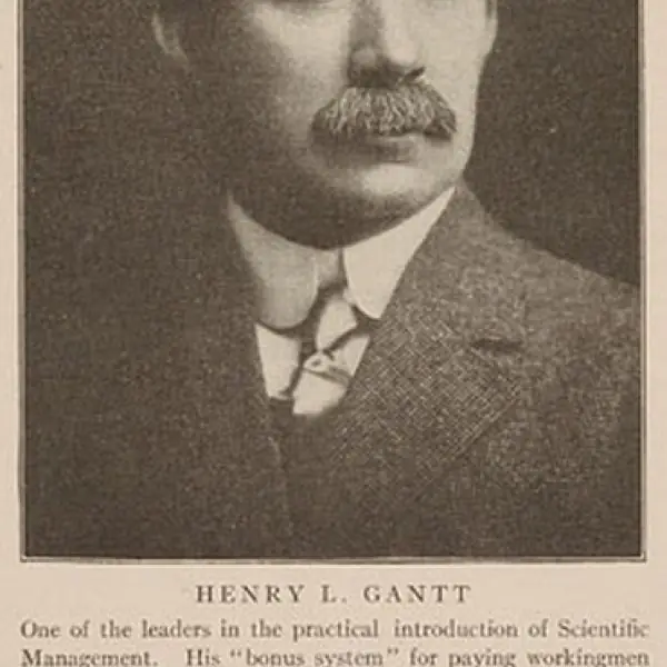
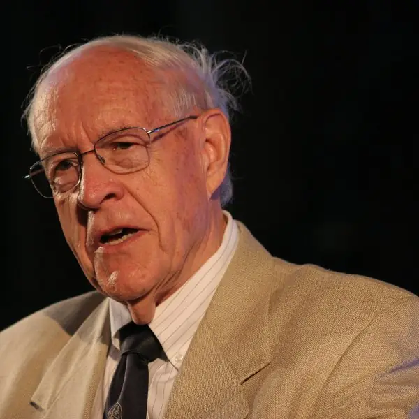
Plate 8.1 shows the two people behind the best-known planning tools and the arithmetic of team size; Figures 8.1 to 8.6 show COCOMO, function points, the critical path, PERT, earned value and risk exposure, all worked with numbers computed by program.


8.7.1 Eight causes of late and over-budget software projects
- Unrealistic estimates. Many projects start with a date chosen by the client and an estimate made to fit it. When COCOMO or function points (Figures 8.1 and 8.2) give a different answer, the honest answer is the number from the model. A wrong estimate guarantees a late project before the first line is written.
- Unclear or changing requirements. If the SRS is incomplete, the team builds the wrong thing and rebuilds it later. Changes without change control add work without adding time. Unit 3 and the change process of Figure 7.5 are the cure.
- Adding people to a late project. Brooks's law says that new staff must be trained and add communication paths, which makes the project later (Plate 8.1). Better remedies are to cut scope, to move the date or to improve the process. This is the commonest mistake of managers under pressure.
- Poor risk management. Risks that were never listed become emergencies. Ranking them by exposure, as in Figure 8.6, directs effort to the real threats. A weekly risk review costs minutes and often saves weeks.
- Weak tracking. If progress is reported as "90 per cent done" nobody can see the truth. Earned value measures, with CPI and SPI (Figure 8.5), show trouble in the first third of the project, when it is still fixable. Regular, honest status reports are essential.
- Ignoring the critical path. A delay in a critical activity delays the whole project, while an activity with slack can slip safely (Figure 8.3). Managers who treat all tasks equally waste effort on the wrong ones. The network shows where to put the best people.
- Weak team and poor communication. Skills mismatch, low morale and unclear roles reduce output more than any tool. Teams of five to nine, a clear leader and short daily meetings keep information flowing. In a distributed team, the written plan matters even more.
- Insufficient testing and quality control. If testing is squeezed to meet the date, faults are found by users after release at about a hundred times the cost (Figure 1.1). Quality gates, reviews and automated tests must be part of the schedule. A project is not finished until it works.
Formula and fact sheet
- Basic COCOMO: E = a·KLOC^b, D = c·E^{d}. Organic 2.4/1.05/2.5/0.38; semi-detached 3.0/1.12/2.5/0.35; embedded 3.6/1.20/2.5/0.32. Intermediate: E = 3.2·KLOC^1.05 × EAF.
- FPA: UFP = Σ count × weight; VAF = 0.65 + 0.01ΣFᵢ; FP = UFP × VAF.
- CPM: ES = max(EF of predecessors); LF = min(LS of successors); slack = LS − ES; critical path = zero slack.
- PERT: tₑ = (o + 4m + p)/6; σ = (p − o)/6; z = (D − μ)/σ.
- EVM: CV = EV − AC; SV = EV − PV; CPI = EV/AC; SPI = EV/PV; EAC = BAC/CPI.
- Risk exposure = probability × loss. Communication paths = n(n − 1)/2.
Chapter summary
- Software projects are hard to manage because the product is intangible, one-off and changing; management comprises planning, scheduling, costing, monitoring, people and risk.
- COCOMO and function points give effort estimates from size or functionality; they are uncertain and should be re-run as knowledge grows.
- CPM finds the critical path and slack; PERT turns three-point estimates into probabilities of meeting a deadline; EVM measures real progress with CPI and SPI and forecasts the final cost.
- Risk is managed by ranking exposure; people and communication determine more projects than tools do.
Practice
- List the main activities of a software project manager.
- Using basic COCOMO (organic: a = 2.4, b = 1.05, c = 2.5, d = 0.38), estimate effort and duration for 32 KLOC.
- Why does an embedded project need more effort than an organic one of the same size?
- Compute unadjusted and adjusted function points for the component counts of Section 8.3 with the stated 14 factor ratings.
- For the activity network of Section 8.4, find the critical path, project duration and the slack of C and E.
- Using PERT, find the probability of finishing the critical path A-B-D-F-G within 20 weeks.
- A project has BAC = 500,000, PV = 250,000, EV = 200,000, AC = 240,000. Compute CPI, SPI, EAC and VAC and interpret.
- Define risk exposure and rank the risks in Section 8.5.
- How many communication paths exist in a team of 8? What does it imply about adding staff to a late project?
Answers and worked solutions
1. Proposal writing, planning and scheduling, costing, monitoring and reviews, personnel selection, reporting and presentations, risk management.
2. E = 2.4 × 32^{1.05} = 91.3 person-months; D = 2.5 × 91.3^{0.38} = 13.9 months; average team E/D = 6.6 people.
3. Embedded systems have tight hardware, timing and reliability constraints, strict verification and little room for trade-offs, modelled by the larger exponent (1.20) and constant (3.6): 230.4 person-months for 32 KLOC against 91.3.
4. UFP = 39 + 33 + 17 + 24 + 12 = 125; ΣFᵢ = 40, VAF = 1.05, FP = 131.25.
5. Critical path A → B → D → F → G; duration 18 weeks; slack of C and E is 4 weeks each (shared).
6. μ = 19.67, σ = 1.700, z = 0.20, probability ≈ 57.8 %.
7. CPI = 200,000/240,000 = 0.833; SPI = 200,000/250,000 = 0.800; EAC = 500,000/0.833 = 600,000; VAC = -100,000. The project is over budget and behind schedule; the forecast overrun is NPR 100,000.
8. RE = probability × loss. Ranking (largest first) is the table in Section 8.5: the top risk is "Estimate too low by 25 %".
9. n(n − 1)/2 = 8 × 7/2 = 28 paths. Each added person adds more paths and needs training, so a late project is delayed further (Brooks's law).
Model answers: medium (5 marks) and long (10 marks) questions
Q1 (5 marks). Explain the basic COCOMO model with its three modes. Calculate the effort and time for a 32 KLOC organic project.
Introduction. The Constructive Cost Model (COCOMO) by Boehm (1981) estimates effort and time from size in thousands of delivered lines of code (KLOC). The basic model is Effort = a (KLOC)^b person-months and Time = 2.5 (Effort)^c months.
- Organic mode. Small teams, familiar problem, relaxed requirements: a = 2.4, b = 1.05, c = 0.38.
- Semi-detached mode. Medium teams, mixed experience: a = 3.0, b = 1.12, c = 0.35.
- Embedded mode. Tight hardware, software and operational constraints: a = 3.6, b = 1.20, c = 0.32.
- Calculation, organic, 32 KLOC. Effort = 2.4 x 32^{1.05} = 91.3 person-months; Time = 2.5 x 91.3^{0.38} = 13.9 months; average staff = 91.3 / 13.9 = 6.6 people.
- Comparison. In Figure 8.1 the same 32 KLOC needs 145.5 pm (semi-detached) and 230.4 pm (embedded), so tight constraints raise the cost by 2.52 times.
Conclusion. COCOMO is a quick, repeatable estimate; it depends on a good size estimate and is better used with a second method such as function points.
Q2 (5 marks). Explain function point analysis. Compute FP for 20 inputs, 12 outputs, 8 inquiries, 6 files and 4 interfaces, all of average complexity, with a total of 42 for the 14 characteristics.
Introduction. Function point analysis (FPA) measures the size of a system from the functions the user sees, not from lines of code, so it can be done from the requirements and does not depend on the language.
- Count five components. External inputs, outputs, inquiries, internal logical files and external interface files.
- Weight each. Average weights are 4, 5, 4, 10 and 7: 20 x 4 + 12 x 5 + 8 x 4 + 6 x 10 + 4 x 7 = 80 + 60 + 32 + 60 + 28 = 260 UFP (Figure 8.2).
- Value adjustment factor. Rate the 14 general system characteristics from 0 to 5 and add: total = 42; VAF = 0.65 + 0.01 x 42 = 1.07.
- Function points. FP = UFP x VAF = 260 x 1.07 = 278.2.
- Use. With about 53 lines of Java per FP the size is about 14,745 lines; the FP count feeds productivity and cost estimates.
Conclusion. FPA is language independent and available early, but the ratings are partly subjective and need trained counters.
Q3 (10 marks). Explain the critical path method and PERT. For the activities of Figure 8.3 compute ES, EF, LS, LF, slack and the critical path, and the probability of finishing within 16 weeks.
Introduction. Project scheduling decides the order and dates of activities.
The critical path method (CPM) uses a network of activities with fixed durations to find the shortest possible project time; PERT adds uncertainty by using three time estimates for every activity.
CPM procedure.
- List the activities, their durations and predecessors.
- Forward pass: ES = the largest EF of the predecessors, EF = ES + duration.
- Backward pass: LF = the smallest LS of the successors (project end for the last activity), LS = LF - duration.
- Slack = LS - ES. Activities with zero slack are critical; the critical path is the longest path and gives the project duration.
Result for Figure 8.3. The project duration is 14 weeks. The critical path is A-B-D-F (3 + 4 + 5 + 2 = 14). Activity C has slack of 4 weeks and E has 2 weeks, so they can slip by that much without delaying the project.
Any delay on A, B, D or F delays the end date one for one.
| Activity | Duration | ES | EF | Slack | Critical |
|---|---|---|---|---|---|
| A | 3 | 0 | 3 | 0 | yes |
| B | 4 | 3 | 7 | 0 | yes |
| C | 2 | 3 | 5 | 4 | no |
| D | 5 | 7 | 12 | 0 | yes |
| E | 3 | 7 | 10 | 2 | no |
| F | 2 | 12 | 14 | 0 | yes |
PERT. For every activity the expected time is te = (o + 4m + p) / 6 and the variance is ((p - o) / 6)^2.
For the critical path A, B, D, F with estimates (2, 3, 4), (3, 4, 7), (4, 5, 8) and (1, 2, 3): the expected time is mu = 3.00 + 4.33 + 5.33 + 2.00 = 14.67 weeks; the variance is 0.111 + 0.444 + 0.444 + 0.111 = 1.111, so sigma = 1.05.
For a deadline of 16 weeks Z = (16 - 14.67) / 1.05 = 1.26, and from the normal table the probability of finishing on time is 89.7% (Figure 8.4).
The expected time (14.67) is longer than the CPM time (14) because the estimates are skewed to the pessimistic side.
| Aspect | CPM | PERT |
|---|---|---|
| Duration | one fixed estimate | three estimates, probabilistic |
| Used for | repeated, known work | uncertain, research-like work |
| Output | critical path and slack | critical path, variance, probability |
Conclusion. The network tells the manager where there is no room for delay, and PERT tells how likely a deadline is to be met.
Q4 (5 marks). Explain earned value management. At week 6 of a 12-week, Rs 10,00,000 project, PV = 5,00,000, EV = 4,00,000 and AC = 4,50,000. Interpret the project status.
Introduction. Earned value management (EVM) combines scope, schedule and cost in one set of measures, so progress is compared with the plan in money terms.
- Definitions. PV (planned value) is the budgeted cost of work scheduled; EV (earned value) is the budgeted cost of work actually done; AC (actual cost) is the money spent.
- Variances. CV = EV - AC = Rs -50,000 (negative: over budget); SV = EV - PV = Rs -1,00,000 (negative: behind schedule).
- Indices. CPI = EV / AC = 0.889: each rupee spent has earned 89 paisa; SPI = EV / PV = 0.8: 80% of the planned work is done.
- Forecast. EAC = BAC / CPI = Rs 11,25,000 and VAC = BAC - EAC = Rs -1,25,000, an expected overrun.
- Action. Find the cause (estimates, rework, staffing), re-plan, and re-negotiate scope or budget while it is still early (Figure 8.5).
Conclusion. A CPI and SPI below 1.0 in the first third of a project predicts an overrun, and the sooner the manager acts, the cheaper it is to recover.
Q5 (10 marks). Explain risk management in software projects: identification, analysis, planning and monitoring. Give examples and rank four risks by exposure.
Introduction. A risk is a possible future event that would harm the project's cost, schedule or quality.
Risk management is the process of identifying risks, assessing them, planning how to deal with them and watching them throughout the project, so that surprises become planned responses.
1. Risk identification. Use checklists, brainstorming and past projects. Typical categories: project risks (staff leaving, schedule), product risks (performance, quality), business risks (market change, funding), as in the examples in Figure 8.6.
2. Risk analysis. Estimate the probability and the impact of each risk, then compute exposure = probability x impact.
For a team in a Nepali software firm: R4 unrealistic schedule 0.5 x 8 = 4.0 weeks; R2 requirement change 0.6 x 6 = 3.6; R1 key developer leaves 0.3 x 10 = 3.0; R3 hardware delayed 0.2 x 4 = 0.8. The ranking is R4, R2, R1, R3.
3. Risk planning. For each important risk choose a strategy: avoidance (change the plan so the risk cannot occur), minimisation (reduce probability or impact), or a contingency plan (what to do if it happens).
Examples: R4, a schedule review and a COCOMO re-estimate; R2, a change-control board and an incremental release; R1, pair programming and documentation so that no person is indispensable; R3, an early order and a spare unit.
| Risk | Exposure | Strategy |
|---|---|---|
| R4 unrealistic schedule | 4.0 | avoid: re-estimate |
| R2 requirement change | 3.6 | minimise: change control |
| R1 key developer leaves | 3.0 | minimise: pair work, documents |
| R3 hardware delayed | 0.8 | contingency: spare unit |
4. Risk monitoring. Review the risk list weekly, watch the indicators (for example, rising number of change requests), update probabilities, and activate contingency plans when triggers occur. Closed risks are removed and new ones added.
Conclusion. Risk management focuses limited effort on the largest exposures; a project with a ranked and monitored risk list is far less likely to be surprised.