Unit 7 · 6 teaching hours · 17 min read
Design of Experiment
What the syllabus asks for 7
- Concept of analysis of variance
- The F statistic and its distribution
- The linear model
- One-way classification
- Two-way classification (one observation per cell)
- Pictures of ANOVA and experimental design
- Eight uses of ANOVA and designed experiments
An experiment deliberately changes conditions to see their effect (three teaching methods, four server configurations, two web page layouts).
Analysis of variance (ANOVA) compares the means of three or more groups at once, which repeated t tests cannot do safely, since each extra test inflates the chance of a false alarm.
- The idea of ANOVA, the F statistic and its distribution.
- The linear model, one-way and two-way classification (fixed effects), with worked ANOVA tables.
7.1 Concept of analysis of variance
The total variation in the data is split into variation between groups (explained by the treatment) and variation within groups (random error).
If treatment means really differ, the between-group variation is large relative to the within-group variation. Null hypothesis H_{0}: all treatment means are equal; H_{1}: at least one differs.
Assumptions: independent observations, normally distributed errors, equal variances.
Basic design principles: randomisation (random assignment of units to treatments), replication (several units per treatment, to estimate error) and blocking/local control (group similar units to remove a nuisance factor).
7.2 The F statistic and its distribution
F = (variance estimate between)/(variance estimate within) = \frac{M S_{b} \mathrm{etween}}{M S_{w} \mathrm{ithin}}, a ratio of two mean squares (each a sum of squares divided by its degrees of freedom).
Under H_{0} it follows the F distribution with (d f_{1} ,\ d f_{2}) degrees of freedom: positively skewed, always ≥ 0, with the shape set by the two df.
Reject H_{0} if F exceeds the critical value F (\alpha ;\ d f_{1} ,\ d f_{2}) (right-tail test). Critical values (\alpha = 0.05): F (2 ,\ 12) = 3.885 ;\ F (2 ,\ 6) = 5.143 ;\ F (3 ,\ 6) = 4.757.
7.3 The linear model
One-way: y_{i} j = \mu + \tau_{i} + \epsilon_{i} j: observation j in treatment i = overall mean + treatment effect (\sum \tau_{i} = 0 in the fixed-effect model, where the treatments are the only ones of interest) + random error \epsilon_{i} j ~ N (0 ,\ \sigma^{2}).
Two-way (one observation per cell, no interaction): y_{i} j = \mu + \alpha_{i} + \beta_{j} + \epsilon_{i} j, with α the row (treatment) effects and β the column (block) effects.
7.4 One-way classification
k groups with n_{i} observations each, total N. Sums of squares: SST = Σ(y − ȳ..)² (total), SSB = Σ n_i(ȳ_i − ȳ..)² (between treatments), \mathrm{SSW} = \mathrm{SST} - \mathrm{SSB} (within, error).
Degrees of freedom: between k - 1; within N - k; total N - 1. Mean squares MSB = SSB/(k − 1), MSW = SSW/(N − k ) ;\ F = MSB/MSW.
Marks: Method A: 82, 85, 88, 90, 85 (mean 86); B: 78, 74, 80, 76, 82 (mean 78); C: 70, 75, 72, 68, 75 (mean 72). N = 15, grand mean = 78.667.
\mathrm{SSB} = 5 (86 - 78.667)^{2} + 5 (78 - 78.667)^{2} + 5 (72 - 78.667)^{2} = 5 (53.78 + 0.444 + 44.44) = 493.33. SST = 609.33; \mathrm{SSW} = 609.33 - 493.33 = 116.00.
| Source | SS | df | MS | F |
|---|---|---|---|---|
| Between methods | 493.33 | 2 | 246.67 | 25.52 |
| Within (error) | 116.00 | 12 | 9.67 | |
| Total | 609.33 | 14 | | |
F = 246.67 / 9.667 = 25.52 > F (2 ,\ 12) = 3.885 (p \approx 0.00005): reject H_{0}: the methods do not all give the same mean marks. ANOVA only says that some means differ; a post-hoc test (Tukey, least significant difference) would say which.
7.5 Two-way classification (one observation per cell)
Rows = a treatments (e.g. crop varieties), columns = b blocks (e.g. fields); one observation in each of the a \times b cells, N = a b.
With grand total G and correction factor C F = \frac{G^{2}}{N}: \mathrm{SST} = \sum y^{2} - C F; \mathrm{SSR} = \frac{\sum (\mathrm{row} \mathrm{totals})^{2}}{b} - C F; \mathrm{SSC} = \frac{\sum (\mathrm{column} \mathrm{totals})^{2}}{a} - C F; \mathrm{SSE} = \mathrm{SST} - \mathrm{SSR} - \mathrm{SSC}.
Degrees of freedom: rows a - 1, columns b - 1, error (a - 1) (b - 1), total a b - 1. F_{r} \mathrm{ows} = MSR/MSE, F_{c} \mathrm{ols} = MSC/MSE.
Blocking removes the column variation from the error, making the treatment test more sensitive.
With m > 1 observations per cell an interaction term (does the row effect depend on the column?) can also be tested, with error df ab(m − 1).
| | B1 | B2 | B3 | B4 | Row total |
|---|---|---|---|---|---|
| V1 | 20 | 22 | 19 | 24 | 85 |
| V2 | 25 | 27 | 25 | 28 | 105 |
| V3 | 18 | 21 | 17 | 21 | 77 |
| Column total | 63 | 70 | 61 | 73 | 267 |
C F = 267^{2} / 12 = 5,940.75. \sum y^{2} = 6,079, so \mathrm{SST} = 138.25. \mathrm{SSR} = \frac{(85^{2} + 105^{2} + 77^{2})}{4} - C F = 6,044.75 − 5,940.75 = 104.00. \mathrm{SSC} = \frac{(63^{2} + 70^{2} + 61^{2} + 73^{2})}{3} - C F = 5,973 − 5,940.75 = 32.25. \mathrm{SSE} = 138.25 - 104 - 32.25 = 2.00.
| Source | SS | df | MS | F | F (0.05) |
|---|---|---|---|---|---|
| Varieties (rows) | 104.00 | 2 | 52.00 | 156.0 | 5.143 |
| Blocks (columns) | 32.25 | 3 | 10.75 | 32.25 | 4.757 |
| Error | 2.00 | 6 | 0.333 | | |
| Total | 138.25 | 11 | | | |
Both F values exceed their critical values: varieties differ significantly, and the blocks differ too, so blocking was worthwhile.
Using software: SPSS Analyze → Compare Means → One-Way ANOVA or General Linear Model → Univariate; Excel Data Analysis → Anova: Single Factor / Two-Factor Without Replication; Python scipy.stats.f_oneway.
7.6 Pictures of ANOVA and experimental design


7.7 Eight uses of ANOVA and designed experiments
- Comparing many means with one test. Three or more groups, such as three teaching methods, can be compared in a single test. Running several t tests would inflate the chance of a false alarm well above 5%. ANOVA keeps the overall error at the stated level.
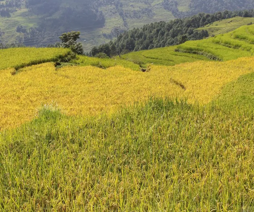
- Choosing the best crop variety or fertiliser. Agricultural stations in Nepal compare paddy or maize varieties on several plots and blocks. ANOVA shows whether the yield differences are real or just soil variation. The blocked design of Figure 7.3 makes the test far more sensitive.
- Comparing algorithms and systems. A developer runs three sorting programs on four data sets and compares the times. The two-way table separates the algorithm effect from the data-set effect. This avoids blaming an algorithm for a hard data set.
- \frac{\frac{A}{B}}{n} testing of products. When a company tests four versions of an a p p screen, one ANOVA tells whether any version differs. Only then is a follow-up test used to find which one. This is cheaper than testing each pair separately.
- Quality control across machines or shifts. A factory compares the output weight of three machines and two shifts. A significant F points to the machine or shift that needs adjusting. Managers can then target the fault instead of retraining everyone.
- Medical and psychological trials. Doses of a drug or kinds of therapy are compared on groups of patients. ANOVA tells whether the treatments differ before doctors study which one is best. Randomisation protects patients from biased allocation.
- Education research. A college compares exam marks across teaching methods, batches or campuses. A significant F supports a change in method; a non-significant one saves money. Section 7.4 works exactly such an example.
- Feature and model selection in data science. The F statistic is used to rank features by how well they separate classes, and to compare the fit of nested regression models. It also underlies the overall F test in regression output. Many software reports show an ANOVA table by default.


Formula and fact sheet
- F = MSB/MSW with (k - 1 ,\ N - k) df; reject if F > F_{c} \mathrm{ritical}.
- One-way: SST = SSB + SSW; SSB = Σn_i(ȳ_i − ȳ)².
- Two-way: C F = \frac{G^{2}}{N} ;\ \mathrm{SSR}, SSC from totals; \mathrm{SSE} = \mathrm{SST} - \mathrm{SSR} - \mathrm{SSC}; error df (a - 1) (b - 1).
- Principles: randomisation, replication, blocking.
Chapter summary
- ANOVA compares several means by splitting total variation into between and within parts and testing their ratio with the F distribution.
- One-way ANOVA handles one factor; two-way ANOVA adds a blocking factor to reduce error.
- A significant F says means differ somewhere; follow-up tests locate the difference.
Practice
- Why can't we simply run several t tests to compare three means?
- Samples A: 6, 8, 7; B: 9, 11, 10; C: 5, 4, 6. Construct the ANOVA table and test at 5% (F (2 ,\ 6) = 5.143).
- State the assumptions of ANOVA.
- Explain randomisation, replication and blocking.
- In a two-way design with 4 rows and 5 columns, give the degrees of freedom of each source.
- What does a significant F-ratio not tell you?
Answers and worked solutions
1. Each test has a 5% chance of a false positive, so repeated testing inflates the overall error rate; ANOVA tests all means with one test.
2. Means 7, 10, 5; grand mean 7.333. \mathrm{SSB} = 3 (0.111 + 7.111 + 5.444) = 38.0; \mathrm{SSW} = (1 + 1 + 0) + (1 + 1 + 0) + (1 + 1 + 0) = 6.0; \mathrm{SST} = 44. \mathrm{MSB} = 19 ,\ \mathrm{MSW} = 1, F = 19.0 > 5.143 → reject H_{0}; the means differ.
3. Independent observations, normal errors, equal variances across groups.
4. Randomisation: assign units to treatments by chance, avoiding bias. Replication: repeat each treatment to estimate error. Blocking: group similar units to remove an unwanted source of variation.
5. Rows 3, columns 4, error 12, total 19.
6. Which means differ, by how much, or whether the differences matter in practice.
Model answers: medium (5 marks) and long (10 marks) questions
Q1 (5 marks). The response times (ms) of three servers, measured four times each, are S1: 14, 16, 15, 17; S2: 19, 21, 20, 22; S3: 12, 13, 15, 12. Construct the one-way ANOVA table and test at the 5% level whether the servers differ. (F (2 ,\ 9) = 4.256 at 5%.)
Introduction. One-way ANOVA tests H_{0}: all group means are equal against H_{1}: at least one differs, by comparing variation between groups with variation within them (Figure 7.1).
Means. S1 = \frac{62}{4} = 15.5; S2 = \frac{82}{4} = 20.5; S3 = \frac{52}{4} = 13.0. N = 12 and the grand mean = 196/12 = 16.333.
Sums of squares. SSB = 4[(15.5 − 16.333)² + (20.5 − 16.333)² + (13 − 16.333)²] = 4(0.694 + 17.361 + 11.111) = 116.67. \mathrm{SST} = \sum (y - 16.333)^{2} = 132.67. \mathrm{SSW} = 132.67 - 116.67 = 16.00.
| Source | SS | df | MS | F |
|---|---|---|---|---|
| Between servers | 116.67 | 2 | 58.33 | 32.81 |
| Within (error) | 16.00 | 9 | 1.778 | |
| Total | 132.67 | 11 |
Decision. F = 58.33 / 1.778 = 32.81 is greater than F (2 ,\ 9) = 4.256, and the p-value is about 0.00007, so reject H_{0}.
Conclusion. The servers do not all have the same mean response time. ANOVA does not say which; a follow-up test (Tukey or least significant difference) would show that S2 is slowest and S3 fastest.
Q2 (5 marks). State the assumptions of ANOVA and explain the three principles of experimental design: randomisation, replication and blocking.
Introduction. The F test is valid only when the data come from a properly designed experiment and meet some conditions.
Assumptions.
- Independence: observations are independent of each other.
- Normality: the errors in each group are approximately normal.
- Equal variances: every group has about the same spread (homogeneity).
- Additivity: in the two-way model, row and column effects simply add up (no interaction).
*Three principles (Figure 7.3 ) . \ast
- Randomisation: treatments are assigned to plots or subjects by chance. It removes selection bias and makes the error terms independent.
- Replication: each treatment is repeated on several units. This allows the error variance to be estimated and gives more precise means.
- Blocking (local control): similar units are grouped into blocks and every treatment appears once in each block. This removes known variation such as soil or batch differences from the error.
Example. To compare three paddy varieties on four fields, plant each variety once in every field (blocking), choose positions at random (randomisation), and use all four fields (replication).
Conclusion A significant F is trustworthy only when these principles were followed.
Q3 (10 marks). Explain two-way ANOVA (one observation per cell). The running times (seconds) of three algorithms on four data sets were: A1: 12, 15, 11, 14; A2: 18, 22, 17, 21; A3: 14, 17, 13, 16. Prepare the ANOVA table and test both effects at 5%. (F (2 ,\ 6) = 5.143 ,\ F ( 3, 6) = 4.757.)
Introduction. Two-way classification studies two factors at once: here algorithms (rows, treatments) and data sets (columns, blocks). The model is y_{i} j = \mu + \alpha_{i} + \beta_{j} + \epsilon_{i} j.
The total variation is split into rows, columns and error, so block-to-block differences are removed from the error and the test of algorithms becomes sharper (Figure 7.4).
Steps.
- Compute the grand total G and correction factor C F = \frac{G^{2}}{N}.
- \mathrm{SST} = \sum y^{2} - C F ;\ \mathrm{SSR} = \frac{\sum (\mathrm{row} \mathrm{totals})^{2}}{b} - C F ;\ \mathrm{SSC} = \frac{\sum (\mathrm{column} \mathrm{totals})^{2}}{a} - C F.
- \mathrm{SSE} = \mathrm{SST} - \mathrm{SSR} - \mathrm{SSC}, with df (a - 1) (b - 1).
- Form the mean squares and the F ratios; compare with the critical values.
Calculation. Row totals: A1 = 52, A2 = 78, A3 = 60. Column totals: 44, 54, 41, 51. G = 190, N = 12. C F = 190^{2} / 12 = 3008.33. \sum y^{2} = 686 + 1538 + 910 = 3134.
\mathrm{SST} = 3134 - 3008.33 = 125.67. \mathrm{SSR} = \frac{(52^{2} + 78^{2} + 60^{2})}{4} - C F = 3097 - 3008.33 = 88.67. \mathrm{SSC} = \frac{(44^{2} + 54^{2} + 41^{2} + 51^{2})}{3} - C F = 3044.67 - 3008.33 = 36.33. \mathrm{SSE} = 125.67 - 88.67 - 36.33 = 0.67.
| Source | SS | df | MS | F | F (0.05) | Decision |
|---|---|---|---|---|---|---|
| Algorithms (rows) | 88.67 | 2 | 44.33 | 399.0 | 5.143 | reject H_{0} |
| Data sets (columns) | 36.33 | 3 | 12.11 | 109.0 | 4.757 | reject H_{0} |
| Error | 0.67 | 6 | 0.111 | |||
| Total | 125.67 | 11 |
One-way versus two-way (Table).
| Point | One-way | Two-way (no replication) |
|---|---|---|
| Factors | one | two (treatment and block) |
| Error df | N - k | (a - 1) (b - 1) |
| Error size | includes block variation | block variation removed |
| F tests | one | two |
| Example | three teaching methods | three algorithms on four data sets |
Interpretation. Both F ratios far exceed their critical values: the algorithms differ in running time, and the data sets differ in difficulty too, so blocking was worthwhile. A2 (mean 19.5 s) is slowest and A1 (13.0 s) fastest.
Conclusion. Two-way ANOVA identified both effects with an error sum of squares of only 0.67. A follow-up multiple-comparison test would confirm which algorithm pairs differ; ANOVA alone says only that the means are not all equal.