Unit 5 · 7 teaching hours · 23 min read
Solution of Ordinary Differential Equations
What the syllabus asks for 9
- Initial value problems
- Taylor series method
- Picard's method
- Euler's method
- Heun's (improved Euler) method
- Runge–Kutta methods
- Higher-order equations and systems
- Boundary value problems and the shooting method
- Seeing the ideas: stepping along slopes, the four slopes of RK4 and how the methods compare
How fast does a cup of tea cool, how does a population grow, how does a capacitor discharge, where does a rocket go? Each is a differential equation, and most have no closed-form solution.
The methods here march forward in small steps from a known starting point, using the equation itself to estimate the slope.
- Initial value problems; Taylor series and Picard's methods.
- Euler's method and its accuracy, Heun's method, Runge–Kutta (RK2, RK4).
- Higher-order equations as first-order systems.
- Boundary value problems and the shooting method.
All tables were generated by bca/tools/check_numerical.py and checked against SciPy's adaptive solver.
5.1 Initial value problems
An initial value problem (IVP) asks for y (x) satisfying y' = f (x ,\ y) ,\ y (x_{0}) = y_{0}. The running example of this unit is
y' = x + y ,\ y (0) = 1, whose exact solution is y = 2 e^{x} - x - 1 (so y (0.5) = 1.797443).
We want approximate values y_{i} \approx y (x_{i}) at x_{i} = x_{0} + ih. A method is single-step if y_{i+1} is computed from y_{i} alone (Euler, Runge–Kutta) and multistep if it also uses earlier values (Adams).
The local truncation error is the error made in one step; the global error is the accumulated error after many steps, typically one power of h lower in order. A method of order p has global error O (h^{p}).
5.2 Taylor series method
Differentiate the equation repeatedly and evaluate at x_{0}: y (x) = y_{0} + (x - x_{0}) y'_{0} + \frac{(x - x_{0})^{2}}{2 !} y''_{0} + \ldots
For y' = x + y ,\ y (0) = 1: y' (0) = 0 + 1 = 1 ;\ y'' = 1 + y' so y'' (0) = 2 ;\ y''' = y'' = 2 ;\ y'''' = 2. Hence
At x = 0.1 four terms give y (0.1) \approx 1.110342 (the true value agrees to six decimals).
At x = 0.5 the same polynomial gives 1.796875, error 0.000568; the error grows as x moves away from 0, so for long intervals the series is used step by step, re-expanding at each new point.
The drawback is that higher derivatives of f (x ,\ y) are tedious to obtain, which is why Runge–Kutta methods were invented.
5.3 Picard's method
Write the IVP as the integral equation y (x) = y_{0} + \int_{x0}^{x} f (t ,\ y (t)) \,d t and iterate: y_{n+1} (x) = y_{0} + \int f (t ,\ y_{n} (t)) \,d t, starting from y_{0} (x) = y_{0}.
For y' = x + y ,\ y (0) = 1:
- y_{1} = 1 + \int_{0}^{x} (t + 1) \,d t = \frac{x^{2}}{2} + x + 1
- y_{2} = 1 + \int_{0}^{x} (t + y_{1} (t)) \,d t = \frac{x^{3}}{6} + x^{2} + x + 1
- y_{3} = \frac{x^{4}}{24} + \frac{x^{3}}{3} + x^{2} + x + 1
Each iteration adds one more correct term of the series 1 + x + x^{2} + \frac{x^{3}}{3} + \frac{x^{4}}{12} + \ldots At x = 0.5 ,\ y_{3} = 1.794271 against the true 1.797443.
Picard iteration proves existence and uniqueness of solutions (under a Lipschitz condition) but is practical only when the integrals can be done analytically.
5.4 Euler's method
Follow the tangent for one step: y_{i+1} = y_{i} + h \cdot f (x_{i} ,\ y_{i}). This is the first two terms of the Taylor series.
| i | x_{i} | y_{i} | f (x_{i} ,\ y_{i}) | y_{i+1} | exact y (x_{i+1}) | error |
|---|---|---|---|---|---|---|
| 0 | 0.0 | 1.000000 | 1.000000 | 1.100000 | 1.110342 | 0.010342 |
| 1 | 0.1 | 1.100000 | 1.200000 | 1.220000 | 1.242806 | 0.022806 |
| 2 | 0.2 | 1.220000 | 1.420000 | 1.362000 | 1.399718 | 0.037718 |
| 3 | 0.3 | 1.362000 | 1.662000 | 1.528200 | 1.583649 | 0.055449 |
| 4 | 0.4 | 1.528200 | 1.928200 | 1.721020 | 1.797443 | 0.076423 |
At x = 0.5 Euler gives 1.721020, the exact value is 1.797443, and the error is 0.076423 (4.3 %). The numerical solution lags behind because the true curve bends upward (convex) and every tangent underestimates it.
Accuracy. The local error is O (h^{2}) (the first dropped Taylor term, \frac{h^{2} y''}{2}) but errors accumulate over \frac{1}{h} steps, so the global error is O (h): halving h halves the error, as the table of Section 5.6 shows.
Euler's method is simple but needs very small steps.
5.5 Heun's (improved Euler) method
Euler uses the slope at the start of the step only. Heun averages the slope at both ends, using Euler to predict the end value:
y \ast = y_{i} + h f (x_{i} ,\ y_{i}) (predictor), y_{i+1} = y_{i} + \left( \frac{h}{2} \right) [f (x_{i} ,\ y_{i}) + f (x_{i+1} ,\ y \ast)] (corrector).
It is the trapezoidal rule applied to the equation, a second-order method with global error O (h^{2}).
| i | x_{i} | y_{i} | predictor y \ast | corrector y_{i+1} | exact |
|---|---|---|---|---|---|
| 0 | 0.0 | 1.000000 | 1.100000 | 1.110000 | 1.110342 |
| 1 | 0.1 | 1.110000 | 1.231000 | 1.242050 | 1.242806 |
| 2 | 0.2 | 1.242050 | 1.386255 | 1.398465 | 1.399718 |
| 3 | 0.3 | 1.398465 | 1.568312 | 1.581804 | 1.583649 |
| 4 | 0.4 | 1.581804 | 1.779985 | 1.794894 | 1.797443 |
At x = 0.5, Heun gives 1.794894 with error 0.002549, about 30 times smaller than Euler's error for the same step.
5.6 Runge–Kutta methods
Runge–Kutta (RK) methods match the Taylor series to a given order without computing derivatives of f, by sampling f at several points inside the step.
RK2 (midpoint/Heun family): k_{1} = f (x_{i} ,\ y_{i}) ,\ k_{2} = f (x_{i} + h ,\ y_{i} + h k_{1}) ,\ y_{i+1} = y_{i} + \left( \frac{h}{2} \right) (k_{1} + k_{2}): this is Heun's method.
Classical RK4 (fourth order, the standard choice):
- k_{1} = f (x_{i} ,\ y_{i})
- k_{2} = f \left( x_{i} + \frac{h}{2} ,\ y_{i} + \frac{h k_{1}}{2} \right)
- k_{3} = f \left( x_{i} + \frac{h}{2} ,\ y_{i} + \frac{h k_{2}}{2} \right)
- k_{4} = f (x_{i} + h ,\ y_{i} + h k_{3})
- y_{i+1} = y_{i} + \left( \frac{h}{6} \right) (k_{1} + 2 k_{2} + 2 k_{3} + k_{4})
It is a Simpson-like weighting: the midpoint slopes count double. Local error O (h^{5}), global O (h^{4}), at the cost of four evaluations of f per step.
First step by hand: k_{1} = f (0 ,\ 1) = 1 ;\ k_{2} = f (0.05 ,\ 1.05) = 1.1 ;\ k_{3} = f (0.05 ,\ 1.055) = 1.105 ;\ k_{4} = f (0.1 ,\ 1.1105) = 1.2105.
The computer gives (1.000000, 1.100000, 1.105000, 1.210500), so y_{1} = 1 + (0.1 / 6) (1 + 2.2 + 2.21 + 1.2105) = 1.110342.
| i | x_{i} | y_{i} | k_{1} | k_{2} | k_{3} | k_{4} | y_{i+1} | exact |
|---|---|---|---|---|---|---|---|---|
| 0 | 0.0 | 1.000000 | 1.000000 | 1.100000 | 1.105000 | 1.210500 | 1.110342 | 1.110342 |
| 1 | 0.1 | 1.110342 | 1.210342 | 1.320859 | 1.326385 | 1.442980 | 1.242805 | 1.242806 |
| 2 | 0.2 | 1.242805 | 1.442805 | 1.564945 | 1.571052 | 1.699910 | 1.399717 | 1.399718 |
| 3 | 0.3 | 1.399717 | 1.699717 | 1.834703 | 1.841452 | 1.983862 | 1.583648 | 1.583649 |
| 4 | 0.4 | 1.583648 | 1.983648 | 2.132831 | 2.140290 | 2.297677 | 1.797441 | 1.797443 |
At x = 0.5, RK4 gives 1.797441; the exact value is 1.797443; the error is only 1.26e-06, with five steps.
Order of accuracy, confirmed
Error at x = 0.5 as the step is halved:
| h | Euler error | Heun error | RK4 error |
|---|---|---|---|
| 0.1 | 7.64e-02 | 2.55e-03 | 1.26e-06 |
| 0.05 | 3.97e-02 | 6.62e-04 | 8.24e-08 |
| 0.025 | 2.02e-02 | 1.69e-04 | 5.26e-09 |
Ratios of error(h = 0.1) / error(h = 0.05): Euler 1.93, Heun 3.85, RK4 15.35. These are close to 2 = 2¹, 4 = 2^{2} ,\ 16 = 2^{4}: the orders 1, 2 and 4.
RK4 with h = 0.1 beats Euler even with h = 0.025 by a factor of thousands, although each step costs four times as much.
Step-size control. Practical solvers (RK45, ode45, SciPy's solve_ivp) compare a fourth- and a fifth-order estimate and adapt h to keep the difference below a tolerance.
Stiff problems (components decaying at very different rates) need implicit methods because explicit ones need tiny steps for stability.
5.7 Higher-order equations and systems
A differential equation of order \ast n \ast converts to \ast n \ast first-order equations. For y'' = g (x ,\ y ,\ y') put z = y':
y' = z ,\ z' = g (x ,\ y ,\ z), with y (x_{0}) and z (x_{0}) = y' (x_{0}) given.
The RK4 formulas are then applied to the vector (y ,\ z): compute k_{1} \ldots k_{4} for each component using the current values of both.
y″ = −y, y(0) = 0, y′(0) = 1 (exact solution y = sin x, z = cos x), RK4, h = 0.1
Writing y' = z ,\ z' = - y. After the first step (y ,\ z) = (0.099833 ,\ 0.995004).
| x | y (RK4) | \sin x | z = y' (RK4) | \cos x |
|---|---|---|---|---|
| 0.1 | 0.099833 | 0.099833 | 0.995004 | 0.995004 |
| 0.2 | 0.198669 | 0.198669 | 0.980067 | 0.980067 |
| 0.3 | 0.295520 | 0.295520 | 0.955337 | 0.955336 |
| 0.4 | 0.389418 | 0.389418 | 0.921061 | 0.921061 |
| 0.5 | 0.479425 | 0.479426 | 0.877583 | 0.877583 |
The five steps reproduce \sin x and \cos x to about six decimals (differences appear in the sixth decimal only), although we used no trigonometry in the method.
5.8 Boundary value problems and the shooting method
In a boundary value problem (BVP) the conditions are given at two points, such as y (a) = \alpha and y (b) = \beta, so we cannot simply march from a known start.
The shooting method guesses the missing initial slope s = y' (a), integrates the IVP to x = b (using RK4), and compares y (b) with the target β.
Treat the miss, \varphi (s) = y (b ;\ s) - \beta, as a function of s and find its root by the secant or bisection methods of Unit 1. For a linear BVP φ is linear in s, so two shots and linear interpolation suffice.
Algorithm. (1) Choose two trial slopes s_{1} ,\ s_{2}. (2) Integrate to get y (b ;\ s_{1}) ,\ y (b ;\ s_{2}). (3) Interpolate: s_{3} = s_{1} + \frac{(\beta - y_{1}) (s_{2} - s_{1})}{(y_{2} - y_{1})}.
(4) Integrate once more with s_{3} and check y (b) = \beta. (For a nonlinear BVP, repeat with the secant formula until |y (b) - \beta| is small.)
Convert to y' = z ,\ z' = y with z (0) = s. Shoot with RK4 (h = 0.1):
| trial | slope s = y' (0) | y (1) by RK4 | target |
|---|---|---|---|
| 1 | 1.0000 | 1.175200 | 2 |
| 2 | 2.0000 | 2.350400 | 2 |
| 3 | 1.701838 | 2.000000 | 2 |
Linear interpolation gives s_{3} = 1.701838; the exact slope is \frac{2}{\sinh 1} = 1.701836, and the third shot hits y (1) = 2.000000. The midpoint value y (0.5) from this slope is 0.886819 against the exact 2 \frac{\sinh (0.5)}{\sinh (1)} = 0.886819.
An alternative is the finite-difference method, which replaces y'' by \frac{y_{i-1} - 2 y_{i} + y_{i+1}}{h^{2}} and solves the resulting linear system (Unit 4); it is more robust for hard problems.
5.9 Seeing the ideas: stepping along slopes, the four slopes of RK4 and how the methods compare
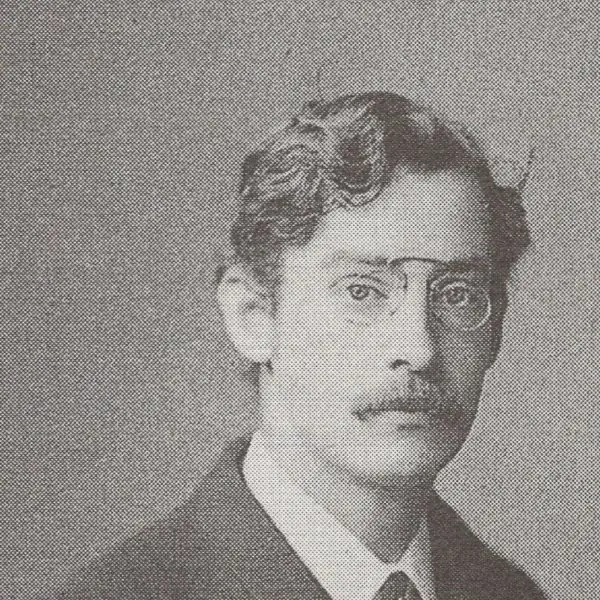
Euler and Runge are the two names behind this unit. Plate 5.1 shows them, together with a picture of the simplest idea in the unit: follow the slope for a short step, then look again.



5.9.1 Eight uses of numerical methods for differential equations
- Weather and climate models. The atmosphere obeys differential equations that cannot be solved exactly. Computers step them forward in small time steps, using methods of Runge-Kutta type. The forecast for the next week is the result of millions of such steps.
- Motion of vehicles and rockets. Position, velocity and fuel change together, and each depends on the others. Engineers integrate the equations step by step to test a flight path before building anything. Satellite orbit prediction works the same way.
- Electric circuits. A circuit with a capacitor or coil is described by a differential equation for charge or current. Simulators such as SPICE solve it numerically for any input signal. Chip designers depend on this.
- Population and epidemic models. The spread of a disease between susceptible and infected people follows coupled equations. Health planners step them forward to compare outcomes of vaccination or lockdown. Planning during the COVID-19 pandemic used models of this kind.
- Chemical reactions and drug dosage. Concentrations change at rates that depend on each other. Numerical solution shows how long a medicine stays active in the body. It guides the dose and the time between doses.
- Cooling, heating and mixing. A cup of tea, a cooling engine and a tank where salt water is mixed all give simple equations that are easy to step. The same method can handle a changing outside temperature, which no formula does. It is a good first exercise.
- Games and animation. Falling objects, springs and cloth in a game are updated each frame by a small step method. A cheap method such as Euler is fast but can drift, so better methods are used for accuracy. Physics engines are made of these steps.
- Finance. Option prices and interest-rate models are described by differential equations that rarely have exact solutions. Banks solve them numerically every day. Accuracy and speed both matter.
Formula and fact sheet
- Euler: y_{i+1} = y_{i} + h f (x_{i} ,\ y_{i}); global error O (h).
- Heun: y \ast = y_{i} + h f ;\ y_{i+1} = y_{i} + \left( \frac{h}{2} \right) [f (x_{i} ,\ y_{i}) + f (x_{i+1} ,\ y \ast)] ;\ O (h^{2}).
- RK4: y_{i+1} = y_{i} + \left( \frac{h}{6} \right) (k_{1} + 2 k_{2} + 2 k_{3} + k_{4}) ;\ O (h^{4}).
- Picard: y_{n+1} = y_{0} + \int f (t ,\ y_{n}) \,d t. Taylor: y = y_{0} + (x - x_{0}) y'_{0} + \ldots
- Higher order: put z = y' and solve the system. Shooting: root of \varphi (s) = y (b ;\ s) - \beta.
Chapter summary
- An IVP is solved by stepping from the initial condition: Taylor and Picard give series; Euler, Heun and RK4 give numbers.
- Euler's method is first order, Heun second, RK4 fourth; halving h reduces the error by about 2, 4 and 16 respectively.
- Higher-order equations become first-order systems.
- BVPs are solved by shooting (guess the slope, integrate, correct with interpolation or secant steps) or by finite differences.
Practice
- For y' = x + y ,\ y (0) = 1 find y (0.1) by the Taylor series using terms up to x^{4}.
- Obtain the third Picard approximation for the same problem.
- Use Euler's method with h = 0.1 to estimate y (0.5) for y' = x + y ,\ y (0) = 1, and find the error against 2 e^{x} - x - 1.
- Do two steps of Heun's method for the same problem.
- Write the RK4 formulas and compute the first step for the same problem with h = 0.1.
- Why is the global error of Euler's method O (h) when its local error is O (h^{2})?
- Convert y'' + y = 0 to a first-order system and do one RK4 step with h = 0.1 from y (0) = 0 ,\ y' (0) = 1.
- Describe the shooting method for y'' = y ,\ y (0) = 0 ,\ y (1) = 2 and give the slope found by two linear-interpolation shots with s = 1 and s = 2.
- How would you check that a numerical ODE solution is accurate?
Answers and worked solutions
1. y = 1 + x + x^{2} + \frac{x^{3}}{3} + \frac{x^{4}}{12} ;\ y (0.1) \approx 1.110342.
2. y_{3} = \frac{x^{4}}{24} + \frac{x^{3}}{3} + x^{2} + x + 1.
3. Euler: y (0.5) \approx 1.721020; exact 1.797443; error 0.076423 (table in Section 5.4).
4. The first two rows of the Heun table in Section 5.5 give y_{1} and y_{2}; Heun is much closer to the exact solution than Euler.
5. k_{1} = f (x ,\ y) ,\ k_{2} = f \left( x + \frac{h}{2} ,\ y + \frac{h k_{1}}{2} \right) ,\ k_{3} = f \left( x + \frac{h}{2} ,\ y + \frac{h k_{2}}{2} \right) ,\ k_{4} = f (x + h ,\ y + h k_{3}) ,\ y_{1} = y_{0} + \left( \frac{h}{6} \right) (k_{1} + 2 k_{2} + 2 k_{3} + k_{4}).
First step: k's = (1.000000 ,\ 1.100000 ,\ 1.105000 ,\ 1.210500) ,\ y_{1} = 1.110342.
6. Each step commits an O (h^{2}) error. Reaching a fixed x takes about \frac{1}{h} steps, so the errors accumulate to about \left( \frac{1}{h} \right) \cdot O (h^{2}) = O (h).
7. y' = z ,\ z' = - y; first step (y ,\ z ) = ( 0.099833, 0.995004) (exact \sin 0.1 = 0.099833 ,\ \cos 0.1 = 0.995004).
8. Replace the BVP by y' = z ,\ z' = y ,\ y (0) = 0 ,\ z (0) = s. Shot 1 (s = 1) gives y (1) = 1.175200, shot 2 (s = 2) gives 2.350400. Interpolating for the target 2 gives s_{3} = 1.701838; the exact slope is 1.701836.
9. Repeat with half the step: the results should agree to the required digits (for RK4 the error should shrink about 16-fold), and compare with a known exact solution or a high-accuracy solver where available.
Model answers: medium (5 marks) and long (10 marks) questions
Q1 (5 marks). Use Euler's method with h = 0.1 to find y (0.5) for \frac{d y}{d x} = x + y ,\ y (0) = 1, and compare with the exact solution y = 2 e^{x} - x - 1.
Formula. y (n + 1) = y (n) + h f (x (n) ,\ y (n)) with f = x + y.
| n | x (n) | y (n) | f = x + y | y (n + 1) = y + 0.1f | Exact y (n + 1) | Error |
|---|---|---|---|---|---|---|
| 0 | 0.0 | 1.00000 | 1.00000 | 1.10000 | 1.11034 | 0.01034 |
| 1 | 0.1 | 1.10000 | 1.20000 | 1.22000 | 1.24281 | 0.02281 |
| 2 | 0.2 | 1.22000 | 1.42000 | 1.36200 | 1.39972 | 0.03772 |
| 3 | 0.3 | 1.36200 | 1.66200 | 1.52820 | 1.58365 | 0.05545 |
| 4 | 0.4 | 1.52820 | 1.92820 | 1.72102 | 1.79744 | 0.07642 |
So Euler gives y (0.5) = 1.72102 against the exact 1.79744, an error of 0.0764 (4.3%) (Figure 5.1). Euler is a first-order method: halving h roughly halves the error.
Conclusion Euler is simple but needs a very small step for accuracy.
Q2 (5 marks). Apply one step of the fourth-order Runge-Kutta method to \frac{d y}{d x} = x + y ,\ y (0) = 1 ,\ h = 0.1.
Formulas. k1 = f ( x 0, y0); k2 = f ( x 0 + \frac{h}{2}, y0 + \frac{h k 1}{2}); k3 = f ( x 0 + \frac{h}{2}, y0 + \frac{h k 2}{2}); k4 = f ( x 0 + h, y0 + h k3); y1 = y0 + (\frac{h}{6} ) ( k 1 + 2k2 + 2k3 + k4).
Calculation. k1 = 0 + 1 = 1. k2 = f (0.05 ,\ 1 + 0.05 x 1) = 0.05 + 1.05 = 1.1. k3 = f (0.05 ,\ 1 + 0.05 x 1.1) = 0.05 + 1.055 = 1.105. k4 = f (0.1 ,\ 1 + 0.1 x 1.105) = 0.1 + 1.1105 = 1.2105.
Then y1 = 1 + (0.1 / 6) (1 + 2.2 + 2.21 + 1.2105) = 1 + (0.1 / 6) (6.6205) = 1.110342.
The exact value is 2 e^{0} . 1 - 0.1 - 1 = 1.110342, so one RK4 step is correct to six decimals (Figure 5.2), while one Euler step gave 1.1.
Conclusion RK4 has error O (h^{4}) and is the standard general-purpose method.
Q3 (10 marks). Compare the Taylor, Euler, Heun (improved Euler) and Runge-Kutta methods for the initial value problem y' = f (x ,\ y) ,\ y (x 0) = y0. Illustrate with y' = x + y ,\ y (0) = 1.
Introduction. Most differential equations have no closed-form solution, so we compute y at the points x0 + h, x0 + 2 h ,\ \ldots by repeated small steps.
All methods in this unit are of this kind; they differ in how many slopes they use per step and hence in order and cost (Plate 5.1).
Taylor series method. Expand y (x + h) = y + h y' + \left( \frac{h^{2}}{2} \right) y'' + \ldots using derivatives obtained by differentiating the equation.
It is accurate but needs analytic derivatives, so it is used mostly for hand calculation and to start other methods.
Euler. y (n + 1) = y (n) + h f (x (n) ,\ y (n)): follow the tangent for one step. Local error O (h^{2}), global error O (h): first order.
Heun (improved Euler). A predictor-corrector: predict y \ast = y + h f (x ,\ y), then correct y (n + 1) = y + \left( \frac{h}{2} \right) [f (x ,\ y) + f (x + h ,\ y \ast)], averaging the slopes at both ends. Second order.
Runge-Kutta (RK4). A weighted average of four slopes per step: y (n + 1) = y + \left( \frac{h}{6} \right) ( k 1 + 2k2 + 2k3 + k4) (Figure 5.2). Fourth order: global error O (h^{4}); no derivatives of f are needed.
Illustration. For y' = x + y ,\ y (0) = 1 ,\ h = 0.1, the exact value y (0.5) = 1.797443 is approximated as follows.
| Method | Slopes per step | Order | y (0.5) | Error |
|---|---|---|---|---|
| Euler | 1 | 1 | 1.721020 | 0.076423 |
| Heun | 2 | 2 | 1.794894 | 0.002549 |
| RK4 | 4 | 4 | 1.797441 | 0.0000013 |
Figure 5.3 shows the gain: moving from Euler to RK4 costs four times as many evaluations but reduces the error by a factor of about 60,000.
Systems and higher-order equations. A higher-order equation such as y'' = f (x ,\ y ,\ y') is rewritten as a system u' = v ,\ v' = f (x ,\ u ,\ v) and each component is stepped together.
Boundary value problems are solved by the shooting method, adjusting the starting slope until the far boundary is met.
Stability and step size. Too large a step can make a method blow up, particularly for stiff problems; the step should be reduced until results stop changing, or an adaptive step controller should be used.
Conclusion. Euler is the simplest and least accurate; Heun is a cheap improvement; RK4 is the usual choice because it gives high accuracy at modest cost.