Unit 4 · 10 teaching hours · 22 min read
Solution of Linear Algebraic Equations
What the syllabus asks for 7
- Gauss elimination
- Gauss–Jordan method and matrix inversion
- LU factorisation
- Iterative methods: Jacobi and Gauss–Seidel
- Ill-conditioning
- Eigenvalues: the power method
- Seeing the ideas: elimination, iteration speed and the geometry of ill-conditioning
Circuit analysis, structural frames, the Google PageRank vector and the normal equations of Unit 2 all lead to systems of linear equations Ax = b, sometimes with thousands of unknowns.
This unit covers direct methods (Gauss elimination, Gauss–Jordan, LU), iterative methods (Jacobi, Gauss–Seidel), the dangers of ill-conditioning, and the power method for eigenvalues.
- Gauss elimination with partial pivoting, Gauss–Jordan inversion, LU factorisation.
- Jacobi and Gauss–Seidel iteration; convergence and diagonal dominance.
- Ill-conditioning and the condition number.
- Eigenvalue estimation by the power method.
Syllabus note. The mirror of the TU CACS252 outline used for this book (see bca/SOURCES.md) lists Units 1, 2, 3, 5, 6 but mentions "Linear Algebraic Equations" in the course description and lab list.
The unit is included here as Unit 4, as in other TU outlines; its 10 hours are the remainder of 45.
4.1 Gauss elimination
Forward elimination converts Ax = b to an upper-triangular system by subtracting multiples m_{ik} = \frac{a_{ik}}{a_{kk}} of the pivot row from the rows below. Back substitution then solves from the last equation upwards.
The cost is about \frac{n^{3}}{3} multiplications.
Partial pivoting. Before eliminating column k, swap the row with the largest |a_{ik}| (i \geq k) into the pivot position. This avoids dividing by a zero or tiny pivot and keeps the multipliers |m| \leq 1, which controls round-off. Always use it on a computer.
Operations (with partial pivoting): swap R1 ↔ R2; m21 = -0.6667; m31 = 0.6667; swap R2 ↔ R3; m32 = 0.2000. The reduced upper-triangular augmented matrix is
| x | y | z | RHS |
|---|---|---|---|
| -3.0000 | -1.0000 | 2.0000 | -11.0000 |
| 0.0000 | 1.6667 | 0.6667 | 4.3333 |
| 0.0000 | 0.0000 | 0.2000 | -0.2000 |
Back substitution: z = - 0.2 / 0.2 = - 1 ;\ y = \frac{4.3333 - 0.6667 (- 1)}{1.6667} = 3 ;\ x = \frac{- 11 + 3 - 2 (- 1)}{- 3} = 2.
The solution is (x ,\ y ,\ z) = (2.0000 ,\ 3.0000 ,\ - 1.0000), which agrees with numpy.linalg.solve. Check in the first original equation: 2 (2) + 3 - (- 1) = 8 ✓.
Singular and inconsistent systems. If a zero pivot remains in a column after trying all rows below, the matrix is singular: either no solution (a row 0 = nonzero) or infinitely many (a row 0 = 0).
The determinant equals the product of the pivots times (−1) to the number of swaps.
4.2 Gauss–Jordan method and matrix inversion
Gauss–Jordan continues eliminating above the pivots too, reducing A to the identity; the right-hand side becomes the solution. Applied to the augmented matrix [A | I] it produces A^{-1}.
[A | I]: R_{1} \leftarrow \frac{R_{1}}{2} gives [1, 0.5 | 0.5 ,\ 0 ] ;\ R_{2} \leftarrow R_{2} - 5 R_{1} gives [0, 0.5 | - 2.5 ,\ 1 ] ;\ R_{2} \leftarrow 2 R_{2} gives [0, 1 | - 5 ,\ 2 ] ;\ R_{1} \leftarrow R_{1} - 0.5 R_{2} gives [1, 0 | 3, −1].
So A^{-1} = \begin{bmatrix} 3 & - 1 \\ - 5 & 2 \end{bmatrix}. Numerical check by NumPy: 3.0000, -1.0000, -5.0000, 2.0000 (row-wise).
Check A \cdot A^{-1} = \begin{bmatrix} 6 - 5 & - 2 + 2 \\ 15 - 15 & - 5 + 6 \end{bmatrix} = I ✓.
Gauss–Jordan costs about \frac{n^{3}}{2}, more than Gauss elimination, so use it for inverses, not for single systems.
4.3 LU factorisation
If no row swaps are needed, A = L U with L unit-lower-triangular (1s on the diagonal, the multipliers below) and U upper-triangular (the result of elimination).
Then Ax = b becomes two cheap triangular solves: Ly = b (forward substitution), Ux = y (back substitution).
Once A is factorised, new right-hand sides cost only O (n^{2}), which is why LU is the workhorse of numerical libraries (with pivoting: P A = L U). The determinant is the product of U's diagonal.
Elimination multipliers: m_{21} = 2 ,\ m_{31} = 4, then m_{32} = 3. So L = [ 1 ,\ 0 ,\ 0 ;\ 2 ,\ 1 ,\ 0 ;\ 4 ,\ 3, 1] and U = [ 2 ,\ 1 ,\ 1 ;\ 0 ,\ 1 ,\ 1 ;\ 0 ,\ 0, 2] (rows separated by semicolons).
Forward substitution Ly = b gives y = (4 ,\ 2 ,\ 2); back substitution Ux = y gives x = (1 ,\ 1 ,\ 1). The determinant is 2 \times 1 \times 2 = 4.
Check LU reproduces A and A x = b in code.
Variants: Crout (U has the unit diagonal), Cholesky A = L L^{T} for symmetric positive-definite matrices (half the work, no pivoting needed).
4.4 Iterative methods: Jacobi and Gauss–Seidel
For large sparse systems direct methods fill in zeros and cost too much. Iterative methods start from a guess and improve it. Solve equation \ast i \ast for x_{i}:
- Jacobi: use only the old iterate x^{(k)} on the right (all components updated "simultaneously").
- Gauss–Seidel: use the newest values as soon as they are available (components updated one after another), so it normally converges about twice as fast.
Convergence. Both converge for any start if A is strictly diagonally dominant (|a_{ii}| > \sum_{j \neq i} |a_{ij}| in every row).
That is sufficient, not necessary; the exact condition is that the iteration matrix has spectral radius below 1. Rearranging the equations so that large coefficients lie on the diagonal often helps.
The matrix is strictly diagonally dominant (10 > 3 ,\ 11 > 5 ,\ 10 > 4 ,\ 8 > 4); the exact solution is (1.0000, 2.0000, -1.0000, 1.0000).
Jacobi (first six sweeps):
| k | x_{1} | x_{2} | x_{3} | x_{4} |
|---|---|---|---|---|
| 0 | 0.0000 | 0.0000 | 0.0000 | 0.0000 |
| 1 | 0.6000 | 2.2727 | -1.1000 | 1.8750 |
| 2 | 1.0473 | 1.7159 | -0.8052 | 0.8852 |
| 3 | 0.9326 | 2.0533 | -1.0493 | 1.1309 |
| 4 | 1.0152 | 1.9537 | -0.9681 | 0.9738 |
| 5 | 0.9890 | 2.0114 | -1.0103 | 1.0214 |
| 6 | 1.0032 | 1.9922 | -0.9945 | 0.9944 |
Gauss–Seidel (first six sweeps):
| k | x_{1} | x_{2} | x_{3} | x_{4} |
|---|---|---|---|---|
| 0 | 0.0000 | 0.0000 | 0.0000 | 0.0000 |
| 1 | 0.6000 | 2.3273 | -0.9873 | 0.8789 |
| 2 | 1.0302 | 2.0369 | -1.0145 | 0.9843 |
| 3 | 1.0066 | 2.0036 | -1.0025 | 0.9984 |
| 4 | 1.0009 | 2.0003 | -1.0003 | 0.9998 |
| 5 | 1.0001 | 2.0000 | -1.0000 | 1.0000 |
| 6 | 1.0000 | 2.0000 | -1.0000 | 1.0000 |
To get all components within 5 \times 10^{-5} of the exact answer Jacobi needs 12 sweeps and Gauss–Seidel 6.
The spectral radius of the iteration matrix is 0.4264 for Jacobi and 0.0898 for Gauss–Seidel; the smaller it is, the faster the convergence.
Because each sweep is cheap (n^{2} operations for a dense matrix, far less for sparse ones), iterative methods win for huge sparse systems.
For x + 3 y = 5 ,\ 4 x + y = 6 (solution (1.1818, 1.2727)), Gauss–Seidel from (0, 0) gives (5.00 ,\ - 14.00) \to (47.00 ,\ - 182.00) \to (551 ,\ - 2198) \to (6599 ,\ - 26390): it diverges because the matrix is not diagonally dominant.
Writing the equations in the other order, 4 x + y = 6 first, gives (1.5000 ,\ 1.1667) \to (1.2083 ,\ 1.2639) \to (1.1840 ,\ 1.2720) \to (1.1820 ,\ 1.2727) \to (1.1818 ,\ 1.2727), which converges.
The two systems are mathematically identical.
4.5 Ill-conditioning
A system is ill-conditioned if tiny changes in A or b cause large changes in x. The culprit is a nearly singular matrix, and no algorithm can repair it; pivoting only avoids additional damage.
x + y = 2 ,\ x + 1.0001y = 2.0001 has the solution (1, 1). Change the right-hand side by 0.0001 to 2.0002: the solution jumps to (0, 2). A change of 0.005 % in one coefficient moved the answer by 100 %.
The two equations describe almost parallel lines, so their intersection point is very sensitive.
The condition number κ(A) = ‖A‖·‖A⁻¹‖ measures the amplification: relative error in x \leq \kappa (A) × relative error in the data.
For the matrix above \kappa = 40002, so a relative data error of 10^{-4} may produce a relative solution error of order one.
The 3 \times 3 Hilbert matrix, with entries \frac{1}{i + j - 1}, has \kappa = 524; it is moderately conditioned for n = 3 but becomes terrible as n grows. Rules of thumb: \kappa \approx 10^{k} loses about k significant digits.
Remedies: scaling, pivoting, higher precision, iterative refinement, or reformulating the problem.
4.6 Eigenvalues: the power method
The power method finds the dominant eigenvalue (largest in magnitude) \lambda_{1} and its eigenvector. Start with any v_{0} (with a component along the dominant eigenvector).
Repeat: w = A v_{k-1} ;\ \lambda_{k} = the entry of w with the largest magnitude; v_{k} = \frac{w}{\lambda_{k}}. Then \lambda_{k} \to \lambda_{1} and v_{k} → eigenvector, at a rate |\frac{\lambda_{2}}{\lambda_{1}}|.
| k | A \cdot v_{k-1} | \lambda_{k} (largest entry) | v_{k} (scaled) |
|---|---|---|---|
| 1 | (-1.0000, 2.0000, -1.0000) | 2.0000 | (-0.5000, 1.0000, -0.5000) |
| 2 | (-2.0000, 3.0000, -2.0000) | 3.0000 | (-0.6667, 1.0000, -0.6667) |
| 3 | (-2.3333, 3.3333, -2.3333) | 3.3333 | (-0.7000, 1.0000, -0.7000) |
| 4 | (-2.4000, 3.4000, -2.4000) | 3.4000 | (-0.7059, 1.0000, -0.7059) |
| 5 | (-2.4118, 3.4118, -2.4118) | 3.4118 | (-0.7069, 1.0000, -0.7069) |
| 6 | (-2.4138, 3.4138, -2.4138) | 3.4138 | (-0.7071, 1.0000, -0.7071) |
| 7 | (-2.4141, 3.4141, -2.4141) | 3.4141 | (-0.7071, 1.0000, -0.7071) |
The eigenvalue estimates climb towards 2 + \sqrt{2} = 3.4142, and the vector towards (- 0.7071 ,\ 1 ,\ - 0.7071) \propto \left( 1 ,\ - \sqrt{2} ,\ 1 \right).
The Rayleigh quotient \frac{v^{T} A v}{v^{T} v} of the final vector gives 3.4142, a faster-converging estimate. The smallest eigenvalue can be found by applying the method to A^{-1} (inverse iteration); shifts find the others.
4.7 Seeing the ideas: elimination, iteration speed and the geometry of ill-conditioning
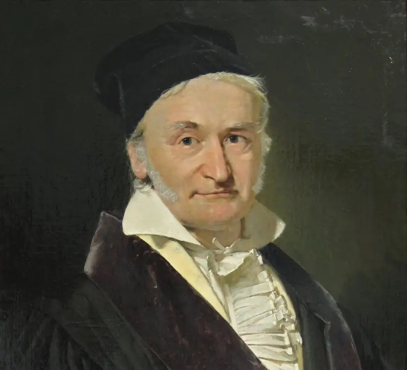
Carl Friedrich Gauss gave elimination its name, and his portrait opens Plate 4.1. The plate also shows why some systems are dangerous: when two lines are nearly parallel, a tiny change moves their intersection a long way.


4.7.1 Eight uses of linear systems and their numerical solution
- Electrical networks. Kirchhoff's laws turn a circuit with many loops into a set of linear equations. A hydropower grid has thousands of nodes and is solved by computer. Elimination or iteration gives all currents at once.
- Structures and bridges. Engineers divide a truss or bridge into joints and write force-balance equations for each. The unknown forces in every member come from one big linear system. The same method checks buildings against earthquake loads.
- Economics and planning. Input-output tables describe how each industry uses the products of others. Solving a linear system shows how much each sector must produce to meet final demand. Governments use it in planning.
- Curve fitting. The normal equations of least squares are linear equations in the unknown coefficients. Every trend line and calibration uses them. A spreadsheet solves them in a moment.
- Computer graphics. Moving, rotating and projecting a 3D model involves solving linear systems for the transformation. Games solve millions of such equations per second. Graphics cards are built for it.
- Search and ranking. The ranking of web pages is an eigenvector problem solved by repeating a matrix multiplication, a method close to the power method. Recommendation systems use the same idea. Linear algebra runs behind the screen.
- Weather and flow simulation. Dividing the air or a river into small cells gives millions of linked equations, solved by fast iterative methods. Direct elimination would be far too slow. Choosing the right method decides whether a forecast arrives in time.
- Network and traffic analysis. Flow of traffic, water in a pipe network and data in a computer network follow balance equations. Solving them locates bottlenecks. Planners in Kathmandu can test a road change on paper first.

Formula and fact sheet
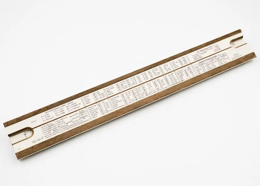
- Multiplier m_{ik} = \frac{a_{ik}}{a_{kk}}; partial pivoting: swap to the largest |a_{ik}| ;\ \det = \pm \Pi pivots.
- Gauss–Jordan on [A | I] gives A^{-1}. LU: Ly = b then Ux = y.
- Jacobi: old values; Gauss–Seidel: newest values; converge if diagonally dominant.
- κ(A) = ‖A‖‖A⁻¹‖; digits lost ≈ \log_{10} \kappa.
- Power method: w = Av, λ = largest entry, v = \frac{w}{\lambda}; rate |\frac{\lambda_{2}}{\lambda_{1}}|.
Chapter summary
- Direct methods (Gauss, Gauss–Jordan, LU) give the exact answer in a fixed number of steps; use partial pivoting.
- Iterative methods suit large sparse systems; Gauss–Seidel usually converges faster than Jacobi, and diagonal dominance guarantees it.
- Ill-conditioned systems amplify data errors regardless of method; the condition number quantifies this.
- The power method estimates the dominant eigenpair using repeated multiplication.
Practice
- Solve 2 x + y - z = 8 ,\ - 3 x - y + 2 z = - 11 ,\ - 2 x + y + 2 z = - 3 by Gauss elimination with partial pivoting.
- Find the inverse of \begin{bmatrix} 2 & 1 \\ 5 & 3 \end{bmatrix} by Gauss–Jordan.
- Factorise A = \begin{bmatrix} 2 & 1 & 1 \\ 4 & 3 & 3 \\ 8 & 7 & 9 \end{bmatrix} as LU and solve Ax = (4, 10, 24).
- Do two Jacobi and two Gauss–Seidel iterations for the 4 \times 4 system of Section 4.4 from zero; which gives the better x_{2}?
- State the sufficient condition for convergence of Jacobi and Gauss–Seidel. Is it necessary?
- Why does Gauss–Seidel diverge for x + 3 y = 5 ,\ 4 x + y = 6 but converge after swapping the equations?
- What is an ill-conditioned system? Illustrate with an example and name the condition number.
- Apply the power method to A = \begin{bmatrix} 2 & - 1 & 0 \\ - 1 & 2 & - 1 \\ 0 & - 1 & 2 \end{bmatrix} and report the eigenvalue after four iterations.
- Compare Gauss elimination and LU factorisation when there are many right-hand sides.
Answers and worked solutions
1. (x ,\ y ,\ z) = (2.0000 ,\ 3.0000 ,\ - 1.0000); the elimination is shown in Section 4.1.
2. A^{-1} = \begin{bmatrix} 3 & - 1 \\ - 5 & 2 \end{bmatrix} (Section 4.2).
3. L = [1 ,\ 0 ,\ 0 ;\ 2 ,\ 1 ,\ 0 ;\ 4 ,\ 3 ,\ 1] ,\ U = [2 ,\ 1 ,\ 1 ;\ 0 ,\ 1 ,\ 1 ;\ 0 ,\ 0 ,\ 2] ,\ y = (4 ,\ 2 ,\ 2) ,\ x = (1 ,\ 1 ,\ 1).
4. From the tables in Section 4.4: after two sweeps Jacobi and Gauss–Seidel give the rows k = 2; Gauss–Seidel's x_{2} = 2.0369 is closer to the exact 2.0000 than Jacobi's value in its table row k = 2, because it uses the new values at once.
5. Strict diagonal dominance of rows: |a_{ii}| > \sum_{j \neq i} |a_{ij}|. It is sufficient but not necessary; convergence actually requires the spectral radius of the iteration matrix to be < 1.
6. In the first order the matrix is not diagonally dominant (|1| < |3|) and the iteration matrix has spectral radius above 1; after swapping, the large entries 4 and 3 sit on the diagonal and the iteration contracts (compare the sequences in Section 4.4).
7. Small input changes cause large output changes, as in x + y = 2 ,\ x + 1.0001y = 2.0001 \to (1 ,\ 1), versus right side 2.0002 \to (0 ,\ 2). The condition number κ(A) = ‖A‖‖A⁻¹‖ (here 40002) measures the amplification.
8. From the table in Section 4.6, the fourth iteration gives \lambda \approx 3.4000 (true 3.4142).
9. Plain elimination repeats the O (n^{3}) work for every new b. LU factorises once (O (n^{3})) and then each right-hand side costs only O (n^{2}) for the two triangular solves.
Model answers: medium (5 marks) and long (10 marks) questions
Q1 (5 marks). Solve 10 x + y + z = 12 ,\ 2 x + 10 y + z = 13 ,\ 2 x + 2 y + 10 z = 14 by Gauss elimination.
Augmented matrix. [10 1 1 | 12; 2 10 1 | 13; 2 2 10 | 14].
*Step 1 (pivot 10 ) . \ast m21 = \frac{2}{10} = 0.2 and m31 = 0.2: R2 = R2 - 0.2R1 gives [0 9.8 0.8 | 10.6]; R3 = R3 - 0.2R1 gives [0 1.8 9.8 | 11.6].
*Step 2 (pivot 9.8 ) . \ast m32 = 1.8 / 9.8 = 0.18367: R3 = R3 - 0.18367R2 gives [0 0 9.6531 | 9.6531] (Figure 4.1).
Back substitution. z = 9.6531 / 9.6531 = 1; y = \frac{10.6 - 0.8 x 1}{9.8} = 1; x = \frac{12 - 1 - 1}{10} = 1.
Check 10 + 1 + 1 = 12 ,\ 2 + 10 + 1 = 13 ,\ 2 + 2 + 10 = 14.
Note with a zero or very small pivot, rows must be swapped (partial pivoting) to keep rounding errors small. The work is about \frac{n^{3}}{3} multiplications.
Conclusion the solution is x = y = z = 1.
Q2 (5 marks). Solve the same system by the Jacobi and Gauss-Seidel methods (four iterations from zero). State the condition for convergence.
Formulas. x = \frac{12 - y - z}{10} ,\ y = \frac{13 - 2 x - z}{10} ,\ z = \frac{14 - 2 x - 2 y}{10}. Jacobi uses only old values of an iteration; Gauss-Seidel uses each new value immediately.
| Iteration | Jacobi (x ,\ y ,\ z) | Gauss-Seidel (x ,\ y ,\ z) |
|---|---|---|
| 1 | 1.2000, 1.3000, 1.4000 | 1.2000, 1.0600, 0.9480 |
| 2 | 0.9300, 0.9200, 0.9000 | 0.9992, 1.0054, 0.9991 |
| 3 | 1.0180, 1.0240, 1.0300 | 0.9996, 1.0002, 1.0000 |
| 4 | 0.9946, 0.9934, 0.9916 | 1.0000, 1.0000, 1.0000 |
Gauss-Seidel is already correct to four decimals after four sweeps, while Jacobi still has an error of 0.008 (Figure 4.2).
Convergence guaranteed when the matrix is strictly diagonally dominant, that is |a (i i)| > sum of |a (i j)| for j not equal i in every row; here 10 > 2 ,\ 10 > 3 and 10 > 4.
Conclusion iterative methods suit large sparse systems and Gauss-Seidel is usually about twice as fast.
Q3 (10 marks). Compare direct and iterative methods for linear systems. Explain LU factorisation and ill-conditioning with an example.
Introduction. To solve Ax = b, direct methods (Gauss elimination, Gauss-Jordan, LU) give the answer after a fixed number of operations, while iterative methods (Jacobi, Gauss-Seidel) improve a guess until it is accurate enough.
Direct methods. Gauss elimination reduces A to upper-triangular form and back-substitutes, with cost about \frac{n^{3}}{3}.
LU factorisation writes A = L U with L lower triangular (holding the multipliers, here 0.2, 0.2, 0.18367) and U upper triangular (the reduced matrix).
To solve for any b, first solve Ly = b by forward substitution, then Ux = y by back substitution, each costing only n^{2}. LU is therefore ideal when the same matrix is used with many right-hand sides.
Gauss-Jordan continues to a diagonal form and can find an inverse but costs more.
Iterative methods. They store only the nonzero entries and need diagonal dominance (Figure 4.2). For a system with a million unknowns, such as a weather grid, they are the only practical choice.
Ill-conditioning. A system is ill-conditioned when small changes in the data cause large changes in the solution (Plate 4.1b).
Example x + y = 2 and x + 1.0001y = 2.0001 has the solution x = 1 ,\ y = 1. Changing the right side to 2.0002 gives y = 0.0002 / 0.0001 = 2 and x = 0: a change of 0.0001 in one datum changed the answer from (1, 1) to (0, 2).
The condition number is \mid |A| \mid x \mid |A^{- 1}| \mid = 2.0001 x 20,001, about 40,000, so relative errors in the data can be magnified up to 40,000 times.
| Point | Direct (LU) | Iterative (Gauss-Seidel) |
|---|---|---|
| Answer after | Fixed steps | Until tolerance met |
| Cost | \frac{n^{3}}{3} | n^{2} per sweep, few sweeps |
| Memory | Fills in zeros | Keeps matrix sparse |
| Condition | Works for any nonsingular A | Needs diagonal dominance |
| Best for | Small and medium systems | Very large sparse systems |
Conclusion. Use LU with partial pivoting for ordinary systems, iterative methods for huge sparse ones, and always check the condition number before trusting an answer.