Depreciation and Inventory Valuation

A delivery van bought for Rs 6,00,000 does not stay worth that amount; it is used up, worn out and eventually sold for scrap.

Depreciation spreads the cost of such an asset over the years that benefit from it, which is the matching concept in action.

The other great judgement in measuring profit is the value placed on unsold goods at year end: inventory valuation. Both change profit without moving any cash, and both are choices governed by standards.

5.1 What depreciation is

Depreciation is the systematic allocation of the depreciable amount of a tangible asset (cost less estimated residual or salvage value) over its useful life. Causes include wear and tear, obsolescence, passage of time and depletion.

It is not a way of setting aside cash and does not measure the asset's market value: it is an allocation of cost.

The standard that governs this (IAS 16, adopted in Nepal as the NFRS for property, plant and equipment) requires that the method reflect the pattern in which the asset's benefits are consumed and that the life and residual value be reviewed at least annually.

5.2 Methods

Straight-line method (SLM): an equal charge each year.

Annual depreciation = (Cost − Residual value) ÷ Useful life.

Written-down-value method (WDV, also reducing-balance): a fixed percentage of the opening book value each year, so the charge is highest at the start. It suits assets whose usefulness or repair cost pattern is front-loaded, and it never reaches exactly zero.

Nepal's Income Tax Act 2058 does not use the accounting method for tax: it groups assets into depreciation pools (blocks) and allows a declining-balance rate per block, for example about 5% for buildings, 25% for computers, furniture and office equipment, 20% for vehicles and construction equipment, and 15% for other assets (verify against the current schedule).

Accounting depreciation per NFRS and tax depreciation per the Act therefore differ, and the difference is carried into a tax computation.

from decimal import Decimal as D, ROUND_HALF_UP
cost, salvage, life = 600000, 60000, 5
slm = (cost - salvage) // life
print(f"SLM annual charge: {slm}")
book = D(cost)
for year in range(1, life + 1):
    dep = (book * D("0.25")).quantize(D("0.01"), ROUND_HALF_UP)
    book -= dep
    print(f"year {year}: WDV charge {dep}, closing {book}")
print(f"year {life} closing WDV: {book}")

SLM annual charge: 108000
year 1: WDV charge 150000.00, closing 450000.00
year 2: WDV charge 112500.00, closing 337500.00
year 3: WDV charge 84375.00, closing 253125.00
year 4: WDV charge 63281.25, closing 189843.75
year 5: WDV charge 47460.94, closing 142382.81
year 5 closing WDV: 142382.81

After five years SLM leaves the van at its residual value of Rs 60,000, while WDV at 25% leaves a book value of Rs 142,382.81. The WDV total charge is smaller in the later years and larger in the early years, so profit is lower early and higher later than under SLM.

5.3 Accounting entries

Direct method: the asset account is credited each year: Dr Depreciation Expense, Cr Asset.

Provision method: the asset stays at cost and the credit goes to an Accumulated Depreciation account: Dr Depreciation Expense, Cr Accumulated Depreciation.

The balance sheet then shows cost, less accumulated depreciation, equals book value (carrying amount). NFRS presentations use the provision method. Depreciation Expense is closed to the Profit and Loss Account at year end.

5.4 Disposal of an asset

When an asset is sold, compute its book value at the date of sale and compare it with the sale proceeds. If proceeds exceed book value, there is a gain; otherwise a loss. The gain or loss goes to the Profit and Loss Account. The entries use an Asset Disposal Account:

1. Transfer the asset's cost: Dr Disposal, Cr Asset.
2. Transfer its accumulated depreciation: Dr Accumulated Depreciation, Cr Disposal.
3. Record the proceeds: Dr Cash or Bank, Cr Disposal.
4. The balancing figure on the disposal account is the gain (credit) or loss (debit), transferred to Profit and Loss.

Depreciation is charged up to the date of sale; a part-year charge is made pro rata by months unless the firm's policy says otherwise.

cost, annual, years_used, proceeds = 600000, 108000, 3, 300000
accumulated = annual * years_used
book_value = cost - accumulated
result = proceeds - book_value
print(f"{'gain' if result >= 0 else 'loss'} on disposal: {abs(result)}")

gain on disposal: 24000

After three years under SLM the accumulated depreciation is Rs 3,24,000 and the book value Rs 276,000. A sale at Rs 3,00,000 produces a gain of Rs 24,000.

5.5 Inventory valuation

Closing inventory is deducted from the goods available for sale to find the cost of goods sold (COGS), so any change in its valuation moves profit by the same amount.

NFRS (IAS 2) requires inventory at the lower of cost and net realisable value (NRV), where NRV is the estimated selling price less the costs to complete and sell.

LIFO is not permitted; the allowed cost formulas are FIFO and weighted average, or specific identification for unique items.

• FIFO (first in, first out): the oldest purchases are assumed sold first, so closing inventory consists of the latest purchases. In rising prices it gives a lower COGS and a higher profit.
• Weighted average cost: each unit carries the average cost of all units available.

from fractions import Fraction
lots = [(100, 50), (200, 55), (150, 60)]
sold = 280
need, cogs = sold, 0
left = []
for qty, price in lots:
    take = min(qty, need)
    cogs += take * price
    need -= take
    if qty > take:
        left.append((qty - take, price))
closing = sum(q * p for q, p in left)
print(f"FIFO: COGS {cogs} closing {closing}")
total_cost = sum(q * p for q, p in lots)
units = sum(q for q, _ in lots)
w_cogs = Fraction(total_cost, units) * sold
print(f"Weighted average: COGS {float(w_cogs):.2f} closing {float(total_cost - w_cogs):.2f}")

FIFO: COGS 14900 closing 10100
Weighted average: COGS 15555.56 closing 9444.44

FIFO gives COGS of Rs 14,900 and closing inventory of Rs 10,100, so gross profit is 22,400 − 14,900 = Rs 7,500.

The weighted average cost per unit is Rs 55.56, giving COGS Rs 15,555.56, closing inventory Rs 9,444.44 and gross profit Rs 6,844.44. In both cases COGS plus closing stock equals Rs 25,000, the goods available.

The choice therefore changes reported profit by Rs 655.56 on the same physical transactions. A firm must apply the chosen method consistently and disclose it; switching merely to improve profit violates the consistency concept.

5.6 Periodic and perpetual systems

In the periodic system, purchases are debited to a Purchases account and inventory is determined by a physical count at period end.

The perpetual system updates inventory after every purchase and sale, so the Inventory account is always current and COGS is recorded at each sale.

The figures above are for a periodic weighted average, because a perpetual average would recompute the average after each receipt and give a slightly different COGS when sales and purchases interleave.

5.7.1 Eight reasons why depreciation and inventory valuation matter

1. Profit becomes fair. A van that serves five years should cost the business a share each year, not all in year 1. Spreading the cost matches expense with the revenue it helps earn. Without depreciation, early profit is too low and later profit too high.
2. Assets are not overstated. Balance-sheet values fall as assets wear out, so the statement is honest. A ten-year-old computer shown at full cost misleads a bank. Book value is cost less accumulated depreciation.
3. Money is set aside in thinking, not in cash. Depreciation is a non-cash expense, so cash does not leave. It warns the owner that the asset must be replaced one day, for example a generator or a delivery bike. Good firms plan that replacement.
4. Tax needs a separate computation. The Income Tax Act uses pools with fixed declining-balance rates, so taxable depreciation differs from the accounting figure. Keeping both records avoids mistakes at filing time. The difference is a normal reconciling item.
5. The method changes profit. SLM and WDV give different charges each year, as the curves show. A firm must choose a method that fits the asset's use and apply it consistently. Changing it only to raise profit breaks the rules.
6. Gain or loss on sale is measured. The book value at the date of sale is compared with the price received. The van sold for Rs 3,00,000 gave a gain of Rs 24,000. The gain or loss goes to the profit and loss account, not to sales.
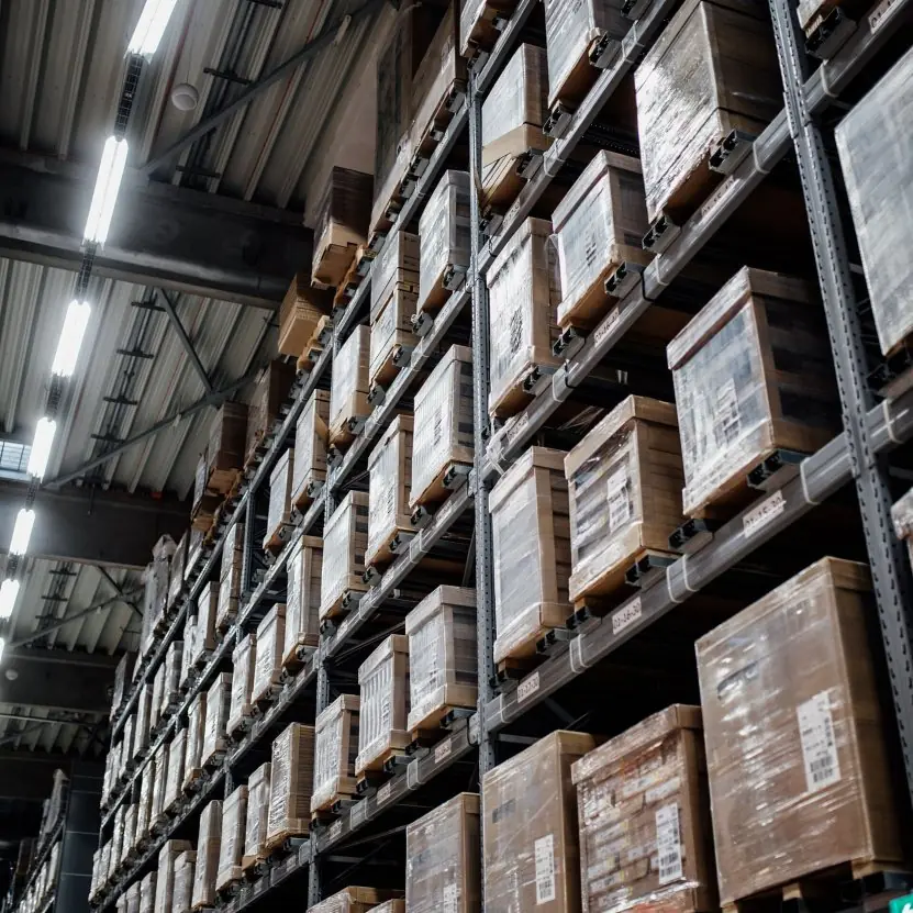
7. Inventory directly sets profit. Closing stock is deducted in finding the cost of goods sold, so every rupee of error in stock is a rupee of error in profit. A warehouse count that misses a rack changes the year's result. Valuation needs care and a physical stock-take.
8. Cost-flow assumptions give different results. FIFO gave a cost of goods sold of Rs 14,900 and the weighted average Rs 15,555.56 on the same units. Inventory is valued at the lower of cost and net realisable value. The method must be disclosed and kept the same year after year.

(a) A Safa tempo, a depreciating asset

(b) Book value after each year, in thousand rupees

5.8 Summary and exercises

Depreciation allocates cost over useful life by SLM or WDV; disposal compares proceeds with book value; inventory is measured at the lower of cost and NRV using FIFO or weighted average, and the method moves profit.

1. Define depreciation and list four causes.
2. A machine costs Rs 4,50,000, residual value Rs 30,000, life 7 years. Prepare the SLM schedule and compute the WDV charge in year 2 at 20%.
3. Journalise depreciation under the direct and provision methods.
4. An asset costing Rs 2,00,000 with Rs 1,20,000 accumulated depreciation is sold for Rs 95,000. Prepare the disposal account.
5. Explain why LIFO is not allowed under NFRS.
6. Using the lots in this unit, compute COGS if 400 units are sold under FIFO.

Model answers: medium (5 marks) and long (10 marks) questions

Q1 (5 marks). Explain depreciation. Compare the straight-line and written-down-value methods for a van costing Rs 6,00,000, residual Rs 60,000, life 5 years, WDV rate 25%.

Depreciation is the systematic allocation of the cost of a tangible asset, less its residual value, over its useful life. It reflects wear, obsolescence and passage of time, and it is a non-cash expense.

SLM. (600,000 − 60,000) ÷ 5 = Rs 1,08,000 each year.

WDV 25% of opening book value: year 1 = 1,50,000; year 2 = 1,12,500; year 3 = 84,375; year 4 = 63,281.25; year 5 = 47,460.94, closing book value Rs 1,42,382.81 (Figure 5.1).

Basis	SLM	WDV
Charge	equal each year	highest first, then falls
Base	original cost less residual	opening book value
Book value at the end	residual value (60,000)	never reaches zero (1,42,382.81)
Suitable for	even-use assets (building)	assets that lose value early (vehicle, computer)
Effect on profit	steady	lower early, higher later

Conclusion. The method must suit the asset and be used consistently.

Q2 (5 marks). The van of Q1 (SLM, 1,08,000 a year) is sold after three years for Rs 3,00,000. Show the disposal account and the gain or loss.

Working. Accumulated depreciation = 1,08,000 × 3 = 3,24,000. Book value = 6,00,000 − 3,24,000 = 2,76,000. Gain = 3,00,000 − 2,76,000 = Rs 24,000 (Figure 5.2).

Dr: Van Disposal A/c	Rs	Cr	Rs
To Van (cost)	6,00,000	By Accumulated depreciation	3,24,000
To Profit and Loss (gain)	24,000	By Bank (proceeds)	3,00,000
	6,24,000		6,24,000

Entries. Dr Disposal and Cr Van 6,00,000; Dr Accumulated Depreciation and Cr Disposal 3,24,000; Dr Bank and Cr Disposal 3,00,000; the balance, a credit of 24,000, is transferred to profit and loss.

If the sale were part-way through a year, the depreciation up to the sale date is charged first.

Conclusion the disposal account shows gain or loss without disturbing sales.

Q3 (10 marks). Explain inventory valuation. Using purchases of 100 units at Rs 50, 200 at Rs 55 and 150 at Rs 60, and a sale of 280 units at Rs 80, compare FIFO and weighted average cost. State the NFRS rule and the periodic and perpetual systems.

Introduction. Closing inventory is deducted from goods available for sale to get the cost of goods sold (COGS), so its valuation changes profit rupee for rupee. NFRS (following IAS 2) requires inventory at the lower of cost and net realisable value (NRV).

Data. 450 units cost Rs 25,000; revenue 280 × 80 = Rs 22,400.

FIFO (Plate 5.1). The 280 units sold are the oldest: 100 × 50 + 180 × 55 = 5,000 + 9,900 = Rs 14,900. Closing: 20 × 55 + 150 × 60 = 1,100 + 9,000 = Rs 10,100. Gross profit = 22,400 − 14,900 = Rs 7,500.

Weighted average. Average cost = 25,000 ÷ 450 = Rs 55.56. COGS = 280 × 55.56 = Rs 15,555.56; closing = 170 × 55.56 = Rs 9,444.44; gross profit = 22,400 − 15,555.56 = Rs 6,844.44.

Measure	FIFO	Weighted average
COGS (Rs)	14,900.00	15,555.56
Closing inventory (Rs)	10,100.00	9,444.44
Gross profit (Rs)	7,500.00	6,844.44
Effect when prices rise	highest profit	profit in the middle

The methods differ by Rs 655.56 on the same units.

Lower of cost and NRV. If goods that cost Rs 10,100 could now be sold for only Rs 9,000 after selling costs, they are shown at Rs 9,000 and the loss of Rs 1,100 is charged at once. This is prudence.

Systems. In the periodic system purchases go to a Purchases account and closing inventory is found by a physical count at the end.

In the perpetual system inventory is updated at every purchase and sale, so COGS and stock are always known; computerised point-of-sale systems use it, and a count still checks for losses.

Consistency. The chosen method must be used every year and disclosed; changing it to raise profit breaches the standards.

Conclusion. FIFO values closing stock at recent prices and gives the higher profit in a period of rising costs; weighted average smooths prices. Whatever method is used, it must be consistent, disclosed and tested against NRV.