Unit 4 · 4 teaching hours · 18 min read
Database Normalization
What the syllabus asks for 9
- Definition and importance
- Functional dependencies
- First normal form (1NF)
- Second normal form (2NF)
- Third normal form (3NF)
- Boyce–Codd normal form (BCNF)
- Fourth normal form (4NF) — multivalued dependencies
- Summary of the normal forms
- Seeing the ideas: anomalies, dependencies and decomposition
Normalization is the process of organising tables to remove redundancy and the update problems that come with it. It is driven by functional dependencies and carried out by decomposing tables into normal forms.
- Why redundancy hurts: insertion, deletion and update anomalies.
- Functional dependencies, closure and finding candidate keys.
- 1NF, 2NF, 3NF, BCNF and 4NF with worked decompositions.
4.1 Definition and importance
Consider one wide table StudentCourse(sid, name, dept, cid, title, marks) storing the student's name and department on every enrolment row.
- Update anomaly: Sita's department appears in many rows; change it in one and the data is inconsistent.
- Insertion anomaly: a new student who has not enrolled cannot be added (cid would be NULL, part of the key).
- Deletion anomaly: deleting Sita's only enrolment also deletes the fact that she exists.
Normalization removes these by splitting the table so each fact is stored once. A good decomposition is lossless (the original can be rebuilt by joining) and ideally dependency preserving.
4.2 Functional dependencies
X → Y (X determines Y) holds in a relation if any two tuples that agree on X also agree on Y. Examples: sid → name; (sid, cid) → marks; cid → title.
Armstrong's axioms: Reflexivity (if Y ⊆ X then X → Y); Augmentation (X → Y ⇒ XZ → YZ); Transitivity (X → Y, Y → Z ⇒ X → Z). Derived: union (X → Y, X → Z ⇒ X → YZ), decomposition, pseudo-transitivity.
A trivial FD has Y ⊆ X. The closure X⁺ is the set of attributes determined by X, computed by repeatedly adding the right side of every FD whose left side is already inside. X is a super key iff X⁺ is all attributes; a candidate key if additionally minimal.
R(A, B, C, D, E) with F = {A → B, BC → D, D → E}. Compute (AC)⁺: start {A, C}; A → B adds B → {A, B, C}; BC → D adds D → {A, B, C, D}; D → E adds E → {A, B, C, D, E} = all.
AC is a super key; A⁺ = {A, B} and C⁺ = {C} are not, so AC is a candidate key (the only one, since A and C appear on no right side and so must be in every key).
4.3 First normal form (1NF)
Every attribute holds a single atomic value; no repeating groups. A table with phone = '9801, 9802' violates 1NF; fix by one row per phone value (or a separate phone table).
4.4 Second normal form (2NF)
A table is in 2NF if it is in 1NF and no non-key attribute depends on part of a composite key (no partial dependency). Only tables with composite keys can violate it.
Enrollment(sid, cid, name, title, marks) with key (sid, cid), FDs: sid → name; cid → title; (sid, cid) → marks. name and title depend on only part of the key. Decompose: Student(sid, name), Course(cid, title), Enrollment(sid, cid, marks).
4.5 Third normal form (3NF)
A table is in 3NF if it is in 2NF and no non-key attribute depends transitively on the key (non-key → non-key). Formally, for every non-trivial X → A: X is a super key, or A is a prime attribute (part of some candidate key).
Student(sid, name, dept_id, dept_name), key sid; FDs: sid → dept_id, dept_id → dept_name. So sid → dept_name transitively. Decompose: Student(sid, name, dept_id) and Department(dept_id, dept_name).
The join on dept_id restores the original (lossless) and both FDs are preserved.
4.6 Boyce–Codd normal form (BCNF)
A table is in BCNF if for every non-trivial FD X → Y, X is a super key. BCNF is stricter than 3NF: it removes the "prime attribute" loophole. Every BCNF table is in 3NF; the converse fails only when a table has overlapping composite candidate keys.
Teaching(student, subject, teacher): each teacher teaches one subject (teacher → subject); a student has one teacher per subject ((student, subject) → teacher). Candidate keys: (student, subject) and (student, teacher).
The FD teacher → subject has a left side that is not a super key, but subject is prime, so the table is in 3NF yet not BCNF. Decompose into TeacherSubject(teacher, subject) and StudentTeacher(student, teacher).
It is lossless, but the FD (student, subject) → teacher is no longer enforceable within one table: BCNF may sacrifice dependency preservation, which is why 3NF is often the practical target.
4.7 Fourth normal form (4NF) — multivalued dependencies
A multivalued dependency X ↠ Y holds when, for each X value, the set of Y values is independent of the other attributes. A table is in 4NF if it is in BCNF and every non-trivial MVD X ↠ Y has X as a super key.
CourseInfo(course, teacher, book): a course has several teachers and several books, independently.
Storing all combinations forces rows such as (DBMS, Ram, Korth), (DBMS, Ram, Elmasri), (DBMS, Hari, Korth), (DBMS, Hari, Elmasri): course ↠ teacher and course ↠ book, but course is not a key.
Decompose: CourseTeacher(course, teacher) and CourseBook(course, book); redundancy disappears.
4.8 Summary of the normal forms
| Form | Removes | Rule |
|---|---|---|
| 1NF | repeating groups, multi-valued cells | atomic values |
| 2NF | partial dependency | non-key depends on the whole key |
| 3NF | transitive dependency | non-key depends on nothing but the key |
| BCNF | every dependency on a non-super-key | every determinant is a super key |
| 4NF | non-trivial multivalued dependency | MVD determinants are super keys |
"The key, the whole key, and nothing but the key." Denormalization (deliberately re-introducing redundancy) is sometimes used in reporting systems for speed, at the price of the anomalies above.
4.9 Seeing the ideas: anomalies, dependencies and decomposition
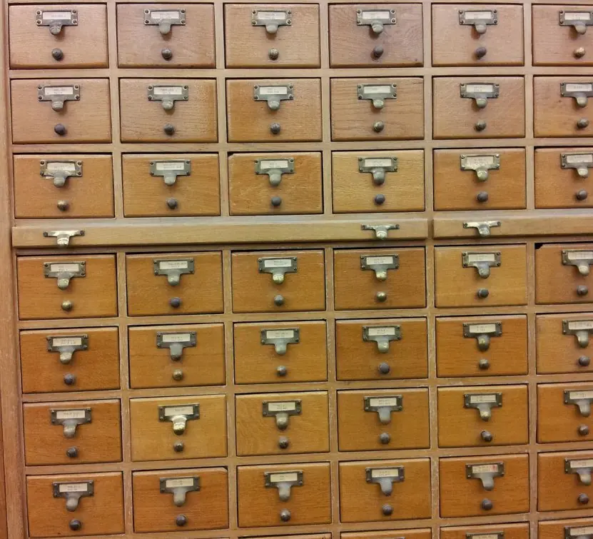
Normalisation is tidying of data, much like a library that keeps one drawer for each subject instead of one huge heap of cards.
The photographs of card drawers remind us that small, well-labelled containers are easier to search, update and keep correct than one large untidy store.
The figures below show the problem (anomalies), the tool (functional dependencies and closure) and the cure (decomposition).


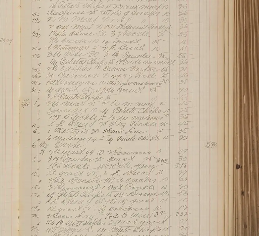
Redundancy used to be visible: an old shop ledger writes the customer's address on every line, and when the customer moves, every line must be corrected.
A flat table does the same thing at a much larger scale, and a DBMS cannot tell which copy is right. The two plates measure the damage on real data and then test a decomposition for the lossless-join property.



4.9.1 Eight advantages of normalisation
- Less redundant data. Each fact, such as the name of a department, is stored once instead of in every student row. A college with ten thousand students saves a great deal of storage. Smaller tables are also faster to scan and to back up.
- No update anomalies. When a department is renamed, one row changes and every student sees the new name. In a flat table a clerk might change two rows and miss a third, leaving the data in contradiction. Normalisation makes such mistakes impossible by design.
- No insertion anomalies. A new department can be recorded before any student joins it, because departments have their own table. In the flat table the department could not exist without a student. This matches how real organisations work.
- No deletion anomalies. If the last student of a department leaves, the fact that the department exists remains. Deleting Hari no longer deletes BIT. Important facts are never lost as a side effect.
- Better data integrity. With one copy of each fact, there is no chance that two copies disagree. Primary and foreign keys then link the pieces, and the DBMS checks the links. Reports from the tables always agree with each other.
- Cleaner, easier design. Each table describes one thing: a student, a course or an enrolment. Designers and programmers find it easy to understand what a table means and where a new column belongs. Documentation and teaching become simpler.
- Easier maintenance and growth. Adding a new attribute to departments touches one small table, not a huge one. Applications that use only students are unaffected. The Nepali university that adds a campus code to its Department table changes one table only.
- Flexible queries. Because data are stored in small logical units, any combination can be rebuilt with a join. A lossless decomposition guarantees that no information is lost when tables are joined again. The same tables can answer questions that nobody planned for at design time.
Formula and fact sheet
- X⁺ = closure; X is a super key iff X⁺ = all attributes.
- Armstrong: reflexivity, augmentation, transitivity.
- 2NF: no partial dependency. 3NF: no transitive dependency (or RHS prime). BCNF: LHS always a super key. 4NF: no non-trivial MVD.
- A lossless decomposition of R into R₁, R₂ needs R₁ ∩ R₂ → R₁ or R₂.
Chapter summary
- Anomalies come from redundancy; normalization removes it by decomposition.
- Closures of attribute sets find keys.
- 1NF (atomic) → 2NF (no partial) → 3NF (no transitive) → BCNF (all determinants keys) → 4NF (no MVD).
Practice
- Define normalization; explain the three anomalies with a table of your own.
- For R(A, B, C, D) with A → B, B → C, C → D find A⁺, B⁺ and the candidate key.
- Normalize Order(oid, date, cid, cname, pid, pname, qty) with key (oid, pid) and FDs oid → date, cid; cid → cname; pid → pname.
- Why is every 2NF violation about a composite key?
- Differentiate 3NF and BCNF with an example.
- State the 4NF rule and give an example of a multivalued dependency.
- Check whether the decomposition of R(A, B, C) with B → C into R₁(A, B), R₂(B, C) is lossless.
Answers and worked solutions
1. Normalization organises tables to remove redundancy using FDs. Anomalies (see 4.1): update (inconsistency), insertion (cannot add a fact without another), deletion (losing one fact loses another).
2. A⁺ = {A, B, C, D} (A→B, B→C, C→D); B⁺ = {B, C, D}. Candidate key: A.
3. 1NF already. Partial dependencies: oid → date, cid; pid → pname. Result: Orders(oid, date, cid), Product(pid, pname), OrderItem(oid, pid, qty). Transitive: cid → cname: Customer(cid, cname), and Orders keeps cid as FK. Final 3NF set: Customer, Orders, Product, OrderItem.
4. A partial dependency is a dependency on part of a key; a single-attribute key has no proper part.
5. 3NF allows X → A when A is prime; BCNF does not. Example: Teaching(student, subject, teacher) in 4.6.
6. 4NF: BCNF plus every non-trivial MVD has a super-key left side. Example: course ↠ teacher with course ↠ book independent.
7. R₁ ∩ R₂ = {B}, and B → C means B is a key of R₂(B, C). So the join on B reproduces R exactly: lossless.
Model answers (5 and 10 marks)
Q1 (5 marks). What is an anomaly? Explain insertion, deletion and update anomalies with an example.
Introduction. An anomaly is an undesirable side effect that appears when a relation stores several facts together, so that one fact is repeated or depends on another.
Consider the flat table StudentDept(sid, name, dept_id, dept_name) with rows (1, Sita, 10, BCA), (2, Ram, 10, BCA) and (3, Hari, 20, BIT), shown in Plate 4.1.
- Update anomaly. The name BCA is stored in two rows. If the department is renamed and only the first row is changed, the table says both BCA and a new name for department 10. The database is inconsistent.
- Insertion anomaly. A new department, 30 BBS, with no students cannot be inserted without a student, because sid is the primary key and cannot be NULL. A true fact cannot be stored.
- Deletion anomaly. Deleting the only student of department 20, Hari, also deletes the fact that department BIT exists. A fact is lost by accident.
- Cause. All three arise from the dependency dept_id → dept_name, where dept_id is not a key of the table (a transitive dependency).
- Cure. Decompose into Student(sid, name, dept_id) and Department(dept_id, dept_name). Each fact is now stored once and the join on dept_id restores the original table.
Conclusion. Anomalies show why redundancy is harmful, and normalisation is the systematic method to remove them.
Q2 (5 marks). Explain 2NF and 3NF with suitable examples.
Introduction. Both normal forms remove dependencies that cause redundancy. They are defined with functional dependencies (FDs); Figure 4.1 shows the examples.
- Second normal form. A relation is in 2NF if it is in 1NF and no non-key attribute depends on a part of a composite key (no partial dependency). Only relations with a composite key can violate it.
- Example. Enrollment(sid, cid, name, title, marks) with key (sid, cid) and FDs sid → name, cid → title, (sid, cid) → marks. Name and title depend on part of the key, so the relation is not in 2NF.
- Decomposition to 2NF. Student(sid, name), Course(cid, title) and Enrollment(sid, cid, marks). Every non-key attribute now depends on the whole key.
- Third normal form. A relation is in 3NF if it is in 2NF and no non-key attribute depends transitively on the key. Formally, for every non-trivial X → A, either X is a super key or A is a prime attribute.
- Example. Student(sid, name, dept_id, dept_name) with sid → dept_id and dept_id → dept_name; dept_name depends on sid only through dept_id.
- Decomposition to 3NF. Student(sid, name, dept_id) and Department(dept_id, dept_name). The decomposition is lossless and preserves both FDs.
Conclusion. A short memory aid is that every non-key attribute depends on the key (1NF), the whole key (2NF) and nothing but the key (3NF).
Q3 (10 marks). What is normalisation? Normalise the relation Registration(sid, cid, name, title, dept_id, dept_name, marks) step by step up to 3NF and compare it with BCNF.
Introduction. Normalisation is the process of decomposing a relation into smaller relations, guided by functional dependencies, so that redundancy and the update, insertion and deletion anomalies are removed while no information is lost.
The relation Registration mixes four facts: students, courses, departments and marks (Figure 4.1).
Step 0: dependencies and key. The FDs are sid → name, dept_id; dept_id → dept_name; cid → title; (sid, cid) → marks.
The closure of (sid, cid) contains all seven attributes (sid, cid, then name, dept_id, dept_name, title, marks), and neither sid nor cid alone does, so the candidate key is (sid, cid).
Step 1: 1NF. Every cell holds one atomic value, and there are no repeating groups, so the relation is already in 1NF. If a cell held two phone numbers it would be split into one row per number.
Step 2: 2NF. Name, dept_id and dept_name depend on sid alone and title depends on cid alone, which are partial dependencies. Decompose into:
- Student(sid, name, dept_id, dept_name)
- Course(cid, title)
- Enrollment(sid, cid, marks)
Step 3: 3NF. In Student the dependency sid → dept_id → dept_name is transitive. Decompose Student into Student(sid, name, dept_id) and Department(dept_id, dept_name).
The final schema is Student, Department, Course and Enrollment, in which every non-key attribute depends on the key, the whole key and nothing but the key.
Step 4: BCNF. A relation is in BCNF if the left side of every non-trivial FD is a super key. In the four final relations the determinants sid, dept_id, cid and (sid, cid) are all keys, so the schema is also in BCNF.
The two forms differ only when a relation has overlapping candidate keys, for example Teaching(student, subject, teacher) with teacher → subject, which is in 3NF but not BCNF.
| Property | 3NF | BCNF |
|---|---|---|
| Rule | non-trivial X → A: X super key or A prime | X must be a super key |
| Redundancy removed | most | all FD-based |
| Always lossless | yes | yes |
| Always dependency-preserving | yes | not always |
Conclusion. The result has no repeated facts and no anomalies, and joining the four tables on sid, dept_id and cid rebuilds Registration exactly. Normalisation costs extra joins, so reporting systems sometimes denormalise deliberately.