Unit 5 · 7 teaching hours · 52 min read
Neural Networks and Natural Language Processing
What the syllabus asks for 7
- The artificial neuron
- The perceptron
- Multi-layer feed-forward networks
- Gradient descent and back-propagation
- Feedback networks: Hopfield network and Boltzmann machine
- Natural language processing
- Seeing the ideas: neurons, perceptrons, networks and language
A human brain has about 86 billion neurons, each a slow, simple cell that adds up signals from thousands of others and fires if the sum is big enough.
Artificial neural networks copy that one idea: a very simple unit, connected in large numbers, with connection strengths learned from data.
This unit builds the model from a single neuron (which can compute AND and OR but provably not XOR) up to multi-layer networks trained by back-propagation, whose arithmetic you will do by hand and the computer will check.
The second half turns to natural language processing: how a program reads, parses and generates human language.
- The artificial neuron, activation functions, the perceptron and its learning rule; gates as neurons.
- Multi-layer feed-forward networks, gradient descent and back-propagation; feedback networks, Hopfield nets and Boltzmann machines.
- Natural language understanding and generation; the steps: lexical, syntactic, semantic, discourse, pragmatic analysis.
- N-gram models, edit distance, TF-IDF, parsing with a grammar.
5.1 The artificial neuron
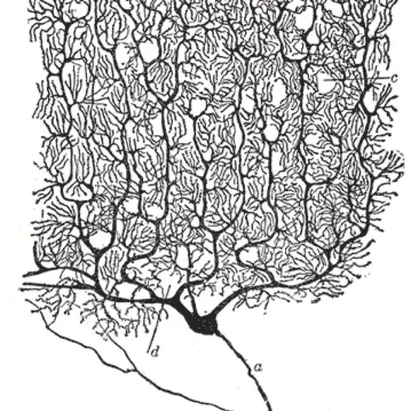
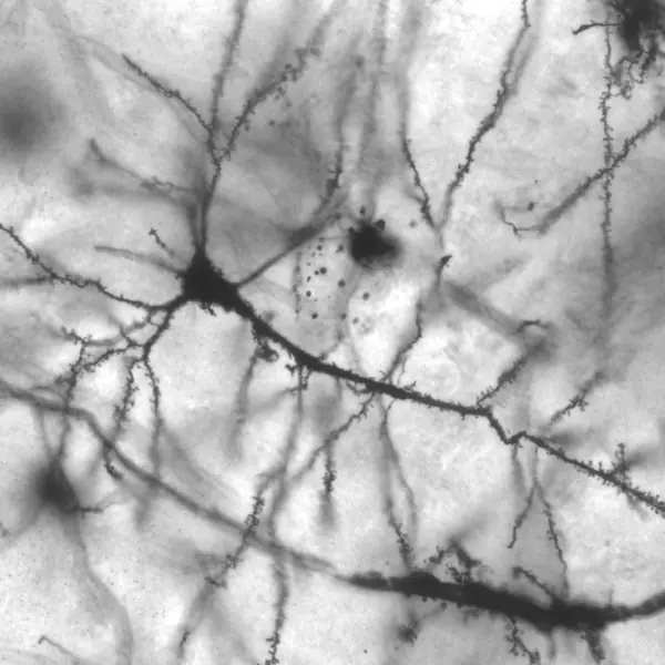
A biological neuron receives signals through dendrites, sums them in the cell body and, when the sum passes a threshold, sends a pulse along the axon to other neurons through synapses, whose strengths change with experience.
McCulloch and Pitts (1943) modelled this as the mathematical neuron:
y = f( Σ wᵢ xᵢ + b )
The inputs xᵢ are multiplied by weights wᵢ, summed with a bias b (a threshold with the sign reversed) and passed through an activation function f.
| Activation | Formula | Range | Use |
|---|---|---|---|
| Step | 1 if z ≥ 0, else 0 | {0, 1} | perceptron |
| Sigmoid | 1 / (1 + e^{-z}) | (0, 1) | probabilities; sigmoid(0) = 0.5, sigmoid(2) = 0.8808 |
| tanh | (e^{z} − e^{-z}) / (e^{z} + e^{-z}) | (−1, 1) | hidden layers; tanh(1) = 0.7616 |
| ReLU | max(0, z) | [0, ∞) | modern deep networks; relu(−2) = 0, relu(3) = 3 |
| Softmax | e^{zᵢ} / Σ e^{zⱼ} | outputs sum to 1 | class probabilities; softmax(2, 1, 0.1) = 0.659, 0.242, 0.099 |
Gate realisation
A single step neuron with suitable weights realises the basic gates. With inputs x₁, x₂ ∈ {0, 1}:
| Gate | w₁ | w₂ | b | Check |
|---|---|---|---|---|
| AND | 1 | 1 | −1.5 | only (1, 1) gives 2 − 1.5 ≥ 0 |
| OR | 1 | 1 | −0.5 | any 1 gives ≥ 0.5 − 0.5 |
| NOT (one input) | −1 | — | 0.5 | x = 0: 0.5 ≥ 0 → 1; x = 1: −0.5 → 0 |
| NAND | −1 | −1 | 1.5 | the complement of AND |
Because NAND is universal, networks of neurons can compute any Boolean function.
5.2 The perceptron
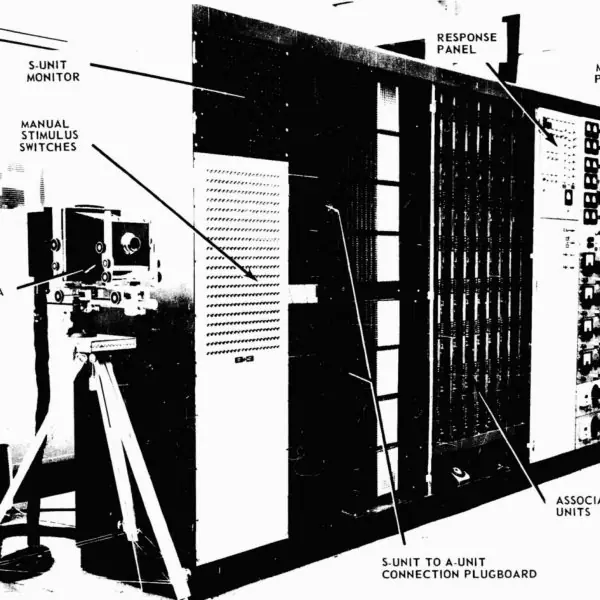
The perceptron (Rosenblatt, 1958) is one step neuron trained by the perceptron learning rule: for each training example with target t and output y, update wᵢ ← wᵢ + η (t − y) xᵢ and b ← b + η (t − y), where η is the learning rate.
Weights change only for misclassified examples.
Training in the order (0,0), (0,1), (1,0), (1,1) with targets 0, 0, 0, 1. The weights at the end of each pass (epoch):
| Epoch | w₁ | w₂ | b | Errors made |
|---|---|---|---|---|
| 1 | 1 | 1 | 0 | 2: (0,0) fired wrongly (z = 0 ≥ 0, so b → −1), and (1,1) was missed |
| 2 | 2 | 1 | −1 | 3 |
| 3 | 2 | 1 | −2 | 3 |
| 4 | 2 | 2 | −2 | 2 |
| 5 | 2 | 1 | −3 | 1 |
| 6 | 2 | 1 | −3 | 0: converged |
The final neuron computes 2x₁ + x₂ − 3 ≥ 0: only (1, 1) gives 0. The perceptron convergence theorem guarantees that this process stops after a finite number of corrections whenever the classes are linearly separable.
The XOR problem
A single perceptron draws a straight line (a hyperplane) in input space, so it can only learn linearly separable functions.
XOR (output 1 when the inputs differ) puts (0, 0) and (1, 1) on one side and (0, 1) and (1, 0) on the other; no line separates them.
The program below trains a perceptron on XOR for 100 epochs: it never converges and never gets more than 2 of the 4 cases right. Minsky and Papert's 1969 book made this point and contributed to the first AI winter. The cure is hidden layers.
5.3 Multi-layer feed-forward networks
A multi-layer perceptron (MLP) has an input layer, one or more hidden layers and an output layer; every neuron feeds the next layer only (feed-forward, no cycles).
With a non-linear activation, one hidden layer with enough neurons can approximate any continuous function (universal approximation theorem).
XOR needs just two hidden neurons: one computing OR, one computing NAND, and the output neuron ANDs them: XOR(x₁, x₂) = AND(OR, NAND).
Types of networks.
Feed-forward signals flow from input to output (MLP, convolutional networks for images). Feedback (recurrent): outputs loop back as inputs, giving memory; used for sequences (RNN, LSTM) and associative memory (Hopfield).
5.4 Gradient descent and back-propagation
Training means choosing weights that minimise a loss E, for example the squared error E = ½ (t − o)² of one example. Gradient descent moves each weight a small step against the gradient: w ← w − η ∂E/∂w.
On E(w) = w² starting at w = 5 with η = 0.1, each step multiplies w by 1 − 2η = 0.8: 4.0, 3.2, 2.56, 2.048, 1.638… If η is too large the steps overshoot and diverge; if too small, learning crawls.
Back-propagation computes ∂E/∂w for every weight efficiently with the chain rule, working from the output back to the input. For a sigmoid neuron, whose derivative is o(1 − o):
- Output neuron error term: δ_o = (o − t) · o (1 − o).
- Hidden neuron j: δⱼ = (Σ_k w_jk δ_k) · hⱼ (1 − hⱼ), the output error passed back through the weights.
- Gradients: ∂E/∂w (weight from neuron i to neuron j) = δⱼ · (output of i). For a bias the "input" is 1.
Algorithm: forward pass; compute the error; backward pass for the δ values; update all weights; repeat for all examples (epochs). Stochastic updates use one example, mini-batch uses a few, batch uses all.
Inputs x = (0.05, 0.10), target t = 1.0, learning rate η = 0.5. Hidden weights: h₁ takes (0.15, 0.20), h₂ takes (0.25, 0.30), both with bias 0.35. Output weights (0.40, 0.45), bias 0.60. All neurons are sigmoid.
Forward: h₁ = σ(0.15·0.05 + 0.20·0.10 + 0.35) = σ(0.3775) = 0.5933; h₂ = σ(0.25·0.05 + 0.30·0.10 + 0.35) = σ(0.3925) = 0.5969; output o = σ(0.40·0.5933 + 0.45·0.5969 + 0.60) = 0.7514. Error E = ½ (1 − 0.7514)² = 0.0309.
Backward: δ_o = (0.7514 − 1) × 0.7514 × 0.2486 = −0.04645. Hidden: δ₁ = δ_o × 0.40 × 0.5933 × 0.4067 = −0.004483; δ₂ = δ_o × 0.45 × 0.5969 × 0.4031 = −0.005029.
Gradients: ∂E/∂w(h₁→o) = δ_o h₁ = −0.02756; ∂E/∂w(h₂→o) = −0.02772; ∂E/∂b_o = −0.04645; for the hidden weights ∂E/∂w = δⱼ xᵢ: −0.000224, −0.000448 (into h₁), −0.000251, −0.000503 (into h₂).
Update (η = 0.5): output weights 0.40 → 0.4138, 0.45 → 0.4639, bias 0.60 → 0.6232; hidden weights 0.15 → 0.1501, 0.20 → 0.2002, 0.25 → 0.2501, 0.30 → 0.3003.
The new forward pass gives o = 0.7588 and E = 0.02909: the error has fallen from 0.0309, as it must for a small step.
The program below also checks every gradient numerically by the finite-difference method; the largest discrepancy is about 10⁻¹¹.
A two-hidden-neuron-plus-one network trained by back-propagation on XOR (three hidden sigmoid units, η = 0.5, 8,000 epochs, random seed 1) produces outputs 0.026, 0.971, 0.972, 0.023 for the inputs 00, 01, 10, 11: the pattern 0, 1, 1, 0 that no single perceptron can learn.
Practical issues
Overfitting (use validation data, early stopping, dropout, weight decay); vanishing gradients (sigmoid saturates, so deep networks use ReLU); local minima; feature scaling; initialisation (random small weights to break symmetry); learning rate schedules.
Deep learning stacks many layers: convolutional networks for images, recurrent networks and transformers for text.
5.5 Feedback networks: Hopfield network and Boltzmann machine
A Hopfield network is a fully connected recurrent network of N bipolar (±1) neurons with symmetric weights and no self-connections. To store patterns p¹, p², … use Hebbian learning: w_ij = Σ_μ p_i^μ p_j^μ (i ≠ j).
To recall, present a noisy pattern and update neurons repeatedly by s_i ← sign(Σ_j w_ij s_j) until nothing changes.
The network always settles into a stable state because an energy E = −½ Σ w_ij s_i s_j never increases; stored patterns are low-energy attractors, so the network is a content-addressable (associative) memory.
Capacity is about 0.14 N random patterns before recall fails.
The program below stores one 8-bit pattern and repairs a copy with two corrupted bits; it then stores a second, orthogonal pattern in the same 8 neurons and shows the recall failing: with N = 8 the capacity rule gives barely one pattern (0.14 × 8 ≈ 1.1), and the crowded network settles into a spurious attractor (the mirror image of the second pattern; the energy function is symmetric under s → −s, so every stored pattern has a mirror twin).
A Boltzmann machine is a Hopfield-like network with stochastic neurons: a neuron turns on with probability 1 / (1 + e^{-\Delta E/T}), and the temperature T is lowered as in simulated annealing so that the network escapes poor local energy minima.
It has hidden units and learns a probability distribution over patterns. The restricted Boltzmann machine (no connections within a layer) was an early building block of deep learning.
5.6 Natural language processing
Natural language processing (NLP) is the AI field that lets computers work with human language.
Natural language understanding (NLU) maps text to a meaning representation (intent, entities, a logical form); natural language generation (NLG) goes the other way, producing text from data or meaning (a weather report from numbers).
Applications: machine translation, speech assistants, search, summarisation, sentiment analysis, spelling and grammar correction, question answering.
Language is hard because it is ambiguous at every level: lexical (bank: river or money), syntactic ("I saw the man with the telescope": who has it?), semantic and pragmatic ("Can you pass the salt?" is a request), and because it needs world knowledge.
Nepali adds Devanagari script, rich inflection (verbs mark person, honorific level and tense), free word order, and few digital resources compared with English.
Steps in natural language processing
- Lexical (morphological) analysis: split text into tokens (words) and reduce them to roots: stemming (chopping suffixes: "running" → "run") or lemmatisation (dictionary form: "better" → "good"); recognise parts of speech.
- Syntax analysis (parsing): find the grammatical structure with a grammar, producing a parse tree; reject ungrammatical sentences.
- Semantic analysis: assign meaning to the structure (word senses, predicate–argument structure, logical form).
- Discourse integration: resolve references across sentences ("Ram met Sita. He gave her a book") and keep context.
- Pragmatic analysis: interpret what the speaker intends in context (a request, a joke, irony).
Syntax analysis with a grammar
A context-free grammar has rules such as S → NP VP, NP → Det N, VP → V NP. A parser decides whether a sentence is derivable and builds the tree.
The CYK algorithm (for grammars in Chomsky normal form) fills a triangular table with the non-terminals that cover each span of words.
With the grammar above and the lexicon the = Det, a = Det, dog = N, cat = N, saw = V, the sentence "the dog saw a cat" is accepted (NP "the dog", VP "saw a cat") and the scrambled "dog the saw cat a" is rejected.
Statistical language models: n-grams
An n-gram model estimates the probability of a word from the previous n − 1 words. For a bigram model P(wₖ | wₖ₋₁) = count(wₖ₋₁ wₖ) / count(wₖ₋₁).
In the toy corpus "I like tea", "I like coffee", "you like tea", "I drink tea" (each wrapped in start and end markers), "I" appears 3 times: twice followed by "like" and once by "drink", so P(like | I) = 2/3 and P(drink | I) = 1/3. "like" appears 3 times, twice followed by "tea", so P(tea | like) = 2/3.
A sentence is scored by multiplying the bigram probabilities: P(I | start) × P(like | I) × P(tea | like) × P(end | tea) = 3/4 × 2/3 × 2/3 × 1 = 1/3 for "I like tea".
Real systems smooth the counts so that unseen bigrams do not get probability zero; modern systems use neural language models (transformers) trained on billions of words.
Text similarity
Edit (Levenshtein) distance is the minimum number of insertions, deletions and substitutions turning one string into another: kitten → sitting is 3 (substitute k→s, e→i, insert g); sunday → saturday is 3; nepal → nepali is 1.
It powers spell-checkers. TF-IDF weights a term by how often it occurs in a document (TF) times how rare it is across documents (IDF = log₁₀(N / df)); a word in every document gets weight 0.
In three documents "the cat sat on the mat", "the dog sat on the log", "cats and dogs": the word the has TF = 2/6 and df = 2, giving 0.0587 in document 1; cat has TF = 1/6 and df = 1, giving 0.0795.
Cosine similarity between the count vectors of "the cat sat" and "the cat ran" is 2/(√3 √3) = 0.6667.
Practising the commands
The first program trains a perceptron on AND (printing the weights after every epoch) and on XOR, and prints the activation values quoted in this unit.
import math
def train(samples, epochs):
    w1 = w2 = b = 0; history = []
    for ep in range(1, epochs + 1):
        errors = 0
        for (x1, x2), t in samples:
            y = 1 if w1 * x1 + w2 * x2 + b >= 0 else 0; e = t - y
            if e: w1 += e * x1; w2 += e * x2; b += e; errors += 1
        history.append((ep, w1, w2, b, errors))
        if errors == 0: break
    return (w1, w2, b), history
AND = [((0, 0), 0), ((0, 1), 0), ((1, 0), 0), ((1, 1), 1)]; XOR = [((0, 0), 0), ((0, 1), 1), ((1, 0), 1), ((1, 1), 0)]
w, hist = train(AND, 20)
for h in hist: print("epoch %d: w1=%d w2=%d b=%d errors=%d" % h)
w, hist = train(XOR, 100)
correct = sum((1 if w[0] * x1 + w[1] * x2 + w[2] >= 0 else 0) == t for (x1, x2), t in XOR)
print("XOR after", len(hist), "epochs: errors in last epoch", hist[-1][4], "correct", correct, "of 4")
sig = lambda z: 1 / (1 + math.exp(-z)); e = [math.exp(v) for v in (2.0, 1.0, 0.1)]
print(round(sig(0), 4), round(sig(2), 4), round(math.tanh(1), 4), [round(v / sum(e), 4) for v in e])
epoch 1: w1=1 w2=1 b=0 errors=2
epoch 2: w1=2 w2=1 b=-1 errors=3
epoch 3: w1=2 w2=1 b=-2 errors=3
epoch 4: w1=2 w2=2 b=-2 errors=2
epoch 5: w1=2 w2=1 b=-3 errors=1
epoch 6: w1=2 w2=1 b=-3 errors=0
XOR after 100 epochs: errors in last epoch 4 correct 2 of 4
0.5 0.8808 0.7616 [0.659, 0.2424, 0.0986]
The second program performs the back-propagation step of this unit, checks the gradients numerically, trains an XOR network and runs the gradient-descent example.
import math, copy, random
sig = lambda z: 1 / (1 + math.exp(-z))
x, t, lr = [0.05, 0.10], 1.0, 0.5
W1 = [[0.15, 0.20], [0.25, 0.30]]; b1 = [0.35, 0.35]; W2 = [0.40, 0.45]; b2 = 0.60
def forward(W1, b1, W2, b2):
    h = [sig(sum(W1[j][i] * x[i] for i in range(2)) + b1[j]) for j in range(2)]
    return h, sig(sum(W2[j] * h[j] for j in range(2)) + b2)
h, o = forward(W1, b1, W2, b2); E = 0.5 * (t - o) ** 2
print("h =", [round(v, 4) for v in h], " o = %.4f  E = %.4f" % (o, E))
d_o = (o - t) * o * (1 - o); d_h = [d_o * W2[j] * h[j] * (1 - h[j]) for j in range(2)]
print("delta_o = %.5f  delta_h = %s" % (d_o, [round(v, 6) for v in d_h]))
gW2 = [d_o * h[j] for j in range(2)]; gW1 = [[d_h[j] * x[i] for i in range(2)] for j in range(2)]
print("grad W2", [round(v, 5) for v in gW2], " grad W1", [[round(v, 6) for v in r] for r in gW1])
def loss(W1, b1, W2, b2): return 0.5 * (t - forward(W1, b1, W2, b2)[1]) ** 2
err = 0
for j in range(2):
    Wp, Wm = copy.deepcopy(W2), copy.deepcopy(W2); Wp[j] += 1e-6; Wm[j] -= 1e-6
    err = max(err, abs((loss(W1, b1, Wp, b2) - loss(W1, b1, Wm, b2)) / 2e-6 - gW2[j]))
    for i in range(2):
        A, B = copy.deepcopy(W1), copy.deepcopy(W1); A[j][i] += 1e-6; B[j][i] -= 1e-6
        err = max(err, abs((loss(A, b1, W2, b2) - loss(B, b1, W2, b2)) / 2e-6 - gW1[j][i]))
print("largest numerical-gradient discrepancy: %.1e" % err)
nW2 = [W2[j] - lr * gW2[j] for j in range(2)]; nW1 = [[W1[j][i] - lr * gW1[j][i] for i in range(2)] for j in range(2)]
nb2 = b2 - lr * d_o; nb1 = [b1[j] - lr * d_h[j] for j in range(2)]
h2, o2 = forward(nW1, nb1, nW2, nb2)
print("new W2", [round(v, 4) for v in nW2], "new b2 %.4f" % nb2, "new W1", [[round(v, 4) for v in r] for r in nW1])
print("after the step: o = %.4f  E = %.5f" % (o2, 0.5 * (t - o2) ** 2))
XOR = [((0, 0), 0), ((0, 1), 1), ((1, 0), 1), ((1, 1), 0)]
rnd = random.Random(1); H = 3
V1 = [[rnd.uniform(-1, 1) for _ in range(2)] for _ in range(H)]; c1 = [rnd.uniform(-1, 1) for _ in range(H)]
V2 = [rnd.uniform(-1, 1) for _ in range(H)]; c2 = rnd.uniform(-1, 1)
for ep in range(8000):
    for (a, b), tt in XOR:
        hh = [sig(V1[j][0] * a + V1[j][1] * b + c1[j]) for j in range(H)]; oo = sig(sum(V2[j] * hh[j] for j in range(H)) + c2)
        d = (oo - tt) * oo * (1 - oo)
        for j in range(H):
            dh = d * V2[j] * hh[j] * (1 - hh[j]); V2[j] -= 0.5 * d * hh[j]
            V1[j][0] -= 0.5 * dh * a; V1[j][1] -= 0.5 * dh * b; c1[j] -= 0.5 * dh
        c2 -= 0.5 * d
print("XOR network outputs:", [round(sig(sum(V2[j] * sig(V1[j][0] * a + V1[j][1] * b + c1[j]) for j in range(H)) + c2), 3) for (a, b), _ in XOR])
w_, trace = 5.0, []
for _ in range(5): w_ -= 0.1 * 2 * w_; trace.append(round(w_, 4))
print("gradient descent on w^2:", trace)
h = [0.5933, 0.5969]  o = 0.7514  E = 0.0309
delta_o = -0.04645  delta_h = [-0.004483, -0.005029]
grad W2 [-0.02756, -0.02772]  grad W1 [[-0.000224, -0.000448], [-0.000251, -0.000503]]
largest numerical-gradient discrepancy: 1.1e-11
new W2 [0.4138, 0.4639] new b2 0.6232 new W1 [[0.1501, 0.2002], [0.2501, 0.3003]]
after the step: o = 0.7588  E = 0.02909
XOR network outputs: [0.026, 0.971, 0.972, 0.023]
gradient descent on w^2: [4.0, 3.2, 2.56, 2.048, 1.6384]
The third program covers the Hopfield network and the language-processing examples (edit distance, bigrams, TF-IDF, cosine similarity and a CYK parser).
import math
p1 = [1, -1, 1, -1, 1, -1, 1, -1]; p2 = [1, 1, 1, 1, -1, -1, -1, -1]; n = 8
def store(*pats): return [[0 if i == j else sum(p[i] * p[j] for p in pats) for j in range(n)] for i in range(n)]
def recall(W, state):
    state = state[:]
    for sweep in range(5):
        for i in range(n): state[i] = 1 if sum(W[i][j] * state[j] for j in range(n)) >= 0 else -1
    return state
noisy = p1[:]; noisy[2] = -noisy[2]; noisy[5] = -noisy[5]
print("noisy", noisy, "differs from p1 in", sum(a != b for a, b in zip(noisy, p1)), "bits")
r1 = recall(store(p1), noisy); print("one pattern stored : recalled == p1:", r1 == p1)
r2 = recall(store(p1, p2), noisy); print("two patterns stored: recalled == p1:", r2 == p1, "| equals -p2:", r2 == [-v for v in p2])
def lev(a, b):
    D = [[i + j if i * j == 0 else 0 for j in range(len(b) + 1)] for i in range(len(a) + 1)]
    for i in range(1, len(a) + 1):
        for j in range(1, len(b) + 1): D[i][j] = min(D[i-1][j] + 1, D[i][j-1] + 1, D[i-1][j-1] + (a[i-1] != b[j-1]))
    return D[-1][-1]
print("edit distances:", lev("kitten", "sitting"), lev("sunday", "saturday"), lev("nepal", "nepali"))
corpus = "<s> i like tea </s> <s> i like coffee </s> <s> you like tea </s> <s> i drink tea </s>".split()
uni, bi = {}, {}
for w in corpus: uni[w] = uni.get(w, 0) + 1
for a, b in zip(corpus, corpus[1:]): bi[(a, b)] = bi.get((a, b), 0) + 1
P = lambda b, a: bi.get((a, b), 0) / uni[a]
print("P(like|i)=%.3f P(drink|i)=%.3f P(tea|like)=%.3f" % (P("like", "i"), P("drink", "i"), P("tea", "like")))
print("P(<s> i like tea </s>) = %.4f" % (P("i", "<s>") * P("like", "i") * P("tea", "like") * P("</s>", "tea")))
docs = ["the cat sat on the mat", "the dog sat on the log", "cats and dogs"]
def tfidf(term, d):
    words = docs[d].split(); df = sum(term in x.split() for x in docs)
    return words.count(term) / len(words) * math.log10(3 / df)
print("tf-idf the@1 %.4f cat@1 %.4f dog@2 %.4f" % (tfidf("the", 0), tfidf("cat", 0), tfidf("dog", 1)))
def cosine(a, b):
    ws = sorted(set(a) | set(b)); u = [a.count(w) for w in ws]; v = [b.count(w) for w in ws]
    return sum(x * y for x, y in zip(u, v)) / (math.hypot(*u) * math.hypot(*v))
print("cosine %.4f" % cosine("the cat sat".split(), "the cat ran".split()))
rules = {("NP", "VP"): "S", ("Det", "N"): "NP", ("V", "NP"): "VP"}; lex = {"the": "Det", "a": "Det", "dog": "N", "cat": "N", "saw": "V"}
def cyk(words):
    n = len(words); T = [[set() for _ in range(n)] for _ in range(n)]
    for i, w in enumerate(words): T[i][i].add(lex[w])
    for span in range(2, n + 1):
        for i in range(n - span + 1):
            j = i + span - 1
            for k in range(i, j):
                for A in T[i][k]:
                    for B in T[k + 1][j]:
                        if (A, B) in rules: T[i][j].add(rules[(A, B)])
    return "S" in T[0][n - 1]
print("CYK:", cyk("the dog saw a cat".split()), cyk("dog the saw cat a".split()))
noisy [1, -1, -1, -1, 1, 1, 1, -1] differs from p1 in 2 bits
one pattern stored : recalled == p1: True
two patterns stored: recalled == p1: False | equals -p2: True
edit distances: 3 3 1
P(like|i)=0.667 P(drink|i)=0.333 P(tea|like)=0.667
P(<s> i like tea </s>) = 0.3333
tf-idf the@1 0.0587 cat@1 0.0795 dog@2 0.0795
cosine 0.6667
CYK: True False
5.7 Seeing the ideas: neurons, perceptrons, networks and language
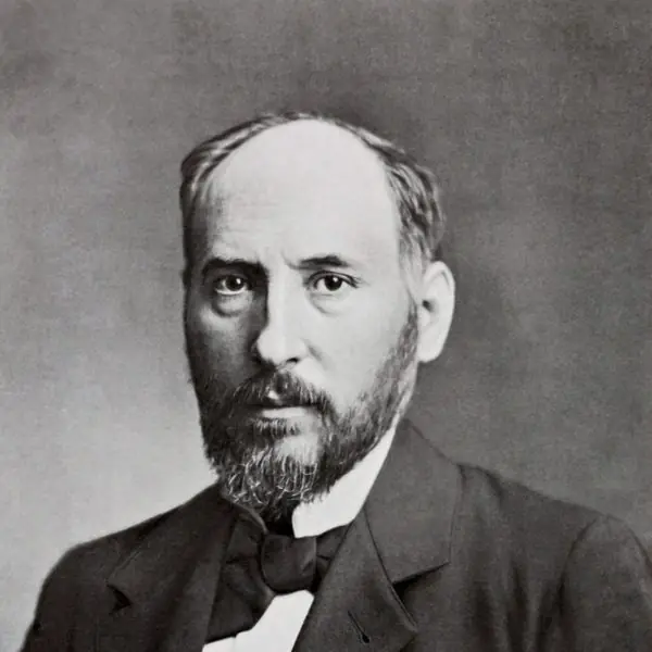
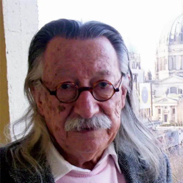
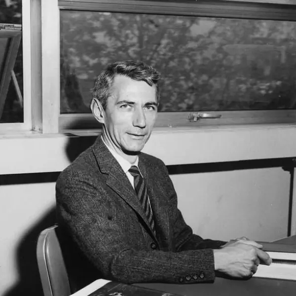
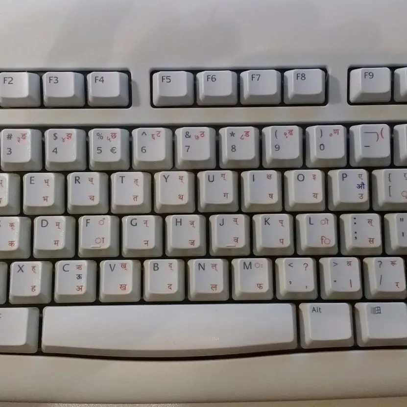
Neural networks and language processing both look mysterious until you watch the numbers move. This section ties each idea to a picture and to a computed figure. Plate 5.1 shows the biological neuron that the model copies.
Plate 5.2 shows the first machine that learned by adjusting weights. Figures 5.1 to 5.7 run the neuron, the perceptron, gradient descent and back-propagation with the same numbers as the text.
Plate 5.3 and Figure 5.8 turn to feedback networks, and Plates 5.4 and 5.5 with Figures 5.9 to 5.12 cover language: levels of analysis, parsing, n-grams, edit distance and TF-IDF.
Every number in a caption was printed by the figure code.
















5.7.1 Eight uses of neural networks and language processing in Nepal
- Reading documents and forms. Land records, citizenship forms and old registers hold handwriting and print that must be typed into computers. A convolutional network, the kind LeCun trained on digits (Plate 5.3), learns to read the characters from many labelled examples. The output is checked by a clerk because a wrong digit in a plot number matters. This saves months of typing in offices that digitise old files.
- Speech and voice search. A neural network turns the sound of Nepali speech into text, so a farmer can search or send a message by speaking. It must be trained on many voices from different districts, because accent changes the sound a great deal. Where training data is scarce the system makes more mistakes, so users should be able to correct it.
- Translation between Nepali and English. Services such as Google Translate learn from texts that exist in both languages, as the Rosetta Stone did with three scripts (Plate 5.4). Government notices, news and study material can be read in either language within seconds. The output still needs a human check for law, medicine and names, because rich Nepali endings (Plate 5.5) are easy to mistranslate.
- Typing help and spell-checking. A phone keyboard suggests the next word from an n-gram model (Fig. 5.11) and fixes a typing error by finding the dictionary word at the smallest edit distance (Fig. 5.12). For Nepali the model must know the verb endings, or it will mark correct forms as errors. Good suggestions make typing in Devanagari faster for students and office workers.
- Chatbots for banks and telecom. A chatbot of a bank, wallet or mobile company must find the intent of a message such as check balance or block card. It follows the levels of Fig. 5.9: split the text, find the structure, find the meaning and keep the context of the chat. Hard cases are handed to a human agent, because a wrong action on an account is costly.
- News search and sentiment. Nepali news portals can rank stories for a search with TF-IDF (Fig. 5.12), so that rare, informative words count more than common ones. A classifier can also tell whether comments on a story are positive or negative. This helps editors see what readers care about, though sarcasm and mixed Nepali-English text confuse it.
- Screening medical images. A convolutional network can look at a chest X-ray or an eye photograph and mark cases that need a doctor first. It is trained on images that specialists have labelled and must be tested on patients from many hospitals, not just one. It supports a health worker in a district hospital who has no specialist at hand, and it never replaces the doctor.
- Identity checks for e-KYC. Banks and wallets that open accounts online compare a selfie with the photograph on the identity document, using a network that turns each face into a list of numbers. If the numbers are close enough the account opens, and if not the case goes to a person. The system must be tested on all kinds of faces and lighting, because errors that fall on one group are unfair.
Formula and fact sheet
- Neuron: y = f(Σ wᵢxᵢ + b). Sigmoid σ(z) = 1/(1 + e^{-z}), σ′ = σ(1 − σ).
- Perceptron rule: w ← w + η(t − y)x. Converges only for linearly separable data; XOR is not.
- Back-propagation: δ_o = (o − t) o (1 − o); δⱼ = (Σ w_jk δ_k) hⱼ(1 − hⱼ); ∂E/∂w = δ · input; w ← w − η ∂E/∂w.
- Hopfield: w_ij = Σ p_i p_j, update s_i = sign(Σ w_ij s_j), capacity ≈ 0.14 N (more patterns give spurious attractors).
- NLP steps: lexical → syntactic → semantic → discourse → pragmatic.
- Bigram P(b | a) = count(ab)/count(a). TF-IDF = tf × log(N/df). Cosine = u·v/(|u||v|).
Chapter summary
- An artificial neuron sums weighted inputs and applies an activation; a perceptron learns linearly separable functions (AND, OR) but not XOR.
- Hidden layers and back-propagation (the chain rule applied layer by layer) let networks learn non-linear functions; training is gradient descent on a loss.
- Hopfield networks store patterns as energy minima and recall them from noisy input while the load stays below about 0.14 N patterns; Boltzmann machines add stochastic units.
- NLP converts text to meaning by lexical, syntactic, semantic, discourse and pragmatic analysis; n-gram, edit-distance and TF-IDF methods are the classical statistical tools.
Practice
- Draw the artificial neuron and give four activation functions.
- Give weights and bias for a single neuron computing AND, OR and NOT. Why can't one neuron compute XOR?
- Train a perceptron on AND with η = 1 from zero weights. Show the weights after epoch 1.
- Construct an XOR network using OR, NAND and AND neurons.
- Define gradient descent. What happens if η is too large?
- For the network of Section 5.4 find δ_o and the new weight from h₁ to the output.
- State the back-propagation algorithm in five steps.
- How does a Hopfield network store and recall patterns? What is its capacity, and what happens above it?
- List and explain the steps of natural language processing.
- Compute the edit distance between "kitten" and "sitting". Why is it useful?
- With the toy corpus of Section 5.6 compute P(like | I) and P(tea | like).
- Distinguish NLU from NLG, and give two ambiguities in language.
Answers and worked solutions
1. Inputs x₁…xₙ with weights w₁…wₙ and a bias b feed a summation and then an activation f. Step, sigmoid, tanh, ReLU (also softmax for outputs).
2. AND: w = (1, 1), b = −1.5. OR: w = (1, 1), b = −0.5. NOT: w = −1, b = 0.5. XOR needs a non-linear boundary; a single neuron separates the plane with one straight line and XOR's two classes are not separable by one.
3. Epoch 1: (0,0) fires wrongly, b → −1; (0,1), (1,0) are correct; (1,1): z = −1 → 0 but t = 1, so w = (1, 1), b = 0. After epoch 1: w = (1, 1), b = 0.
4. Hidden neuron 1 = OR(x₁, x₂), hidden neuron 2 = NAND(x₁, x₂), output = AND(h₁, h₂). For (1, 0): OR = 1, NAND = 1, AND = 1. For (1, 1): OR = 1, NAND = 0, AND = 0.
5. Repeatedly move weights by −η × gradient of the loss. If η is too large the steps overshoot the minimum and the loss oscillates or diverges.
6. δ_o = (0.7514 − 1) × 0.7514 × (1 − 0.7514) = −0.04645. The gradient for the h₁ → output weight is δ_o h₁ = −0.02756, so the new weight is 0.40 − 0.5 × (−0.02756) = 0.4138.
7. (1) Forward pass to get outputs; (2) compute the loss; (3) compute δ at the output; (4) propagate δ backwards through the weights to the hidden layers; (5) update every weight by −η δ × input; repeat.
8. Store by w_ij = Σ p_i p_j (no self-connections); recall by repeated updates s_i = sign(Σ w_ij s_j) from a noisy pattern until stable; capacity is about 0.14 N patterns; above it recall fails and the network settles into spurious attractors (as the 8-neuron example with two patterns showed).
9. Lexical analysis (tokens, stems), syntactic analysis (parse tree), semantic analysis (meaning), discourse integration (reference across sentences), pragmatic analysis (intent in context).
10. 3 (k→s, e→i, insert g). It measures how different two strings are, which is the basis of spelling correction and fuzzy matching.
11. "I" occurs 3 times, followed by "like" twice: P(like | I) = 2/3. "like" occurs 3 times, followed by "tea" twice: P(tea | like) = 2/3.
12. NLU maps text to meaning; NLG produces text from data or meaning. Ambiguities: lexical (bank), syntactic (saw the man with the telescope), pragmatic (Can you pass the salt?).
Model answers for Unit 5
Q1. Describe the artificial neuron. Explain four activation functions and show how single neurons realise AND, OR and NOT. (10 marks)
Introduction. An artificial neuron is the basic unit of a neural network.
It copies the biological neuron, which collects signals through dendrites, adds them in the cell body and, if the total passes a threshold, sends a pulse along the axon.
McCulloch and Pitts (1943) turned this into the model y = f(Σ wᵢxᵢ + b).
Parts (Fig. 5.1). The inputs xᵢ are multiplied by weights wᵢ, which play the role of synapse strengths.
The products are added to a bias b, which is a threshold with its sign reversed, to give z. The activation function f turns z into the output y. For inputs 1, 0.5 and −1, weights 0.4, 0.6, 0.2 and bias −0.1 we get z = 0.4 and, with a sigmoid, y = 0.5987.
| Activation | Formula | Range | Use |
|---|---|---|---|
| Step | 1 if z ≥ 0, else 0 | 0 or 1 | perceptron |
| Sigmoid | 1 / (1 + e^{-z}) | 0 to 1 | probabilities; sigmoid(2) = 0.8808 |
| tanh | (e^{z} − e^{-z}) / (e^{z} + e^{-z}) | −1 to 1 | hidden layers; tanh(1) = 0.7616 |
| ReLU | max(0, z) | 0 upward | deep networks; relu(−2) = 0 |
Gates as neurons (Fig. 5.2). With a step activation and inputs 0 or 1: AND uses weights 1, 1 and bias −1.5, so only (1, 1) gives 2 − 1.5 ≥ 0. OR uses 1, 1 and −0.5, so any input of 1 is enough.
NOT uses weight −1 and bias 0.5: x = 0 gives 0.5 and output 1, x = 1 gives −0.5 and output 0. NAND uses −1, −1 and 1.5. Each is one straight line in the input plane.
Limit. A single neuron cannot compute XOR. Because NAND is universal, a network of neurons can compute any Boolean function.
Conclusion. The neuron is a weighted sum followed by a non-linear function; learning means choosing the weights and the bias.
Q2. State the perceptron learning rule and train a perceptron on AND. What is its limitation? (5 marks)
The perceptron (Rosenblatt, 1958) is one step neuron trained by the rule wᵢ ← wᵢ + η (t − y) xᵢ and b ← b + η (t − y), where t is the target, y the output and η the learning rate. The weights change only when the output is wrong.
Training AND (Fig. 5.3). Take η = 1, start with w = (0, 0), b = 0 and use the order (0,0), (0,1), (1,0), (1,1) with targets 0, 0, 0, 1.
The weights at the end of each epoch are (1, 1, 0), (2, 1, −1), (2, 1, −2), (2, 2, −2), (2, 1, −3) and (2, 1, −3), with 2, 3, 3, 2, 1 and 0 mistakes. The sixth epoch has no mistakes, so training stops.
The final neuron is 2x₁ + x₂ − 3 ≥ 0, which fires only for (1, 1).
Convergence. The perceptron convergence theorem says that the rule stops after a finite number of corrections whenever the classes are linearly separable.
Limitation. One perceptron draws one straight line, so it can learn only linearly separable functions. XOR is not one of them: it never converges and gets at most 2 of the 4 cases right. Minsky and Papert's 1969 book pointed this out. The remedy is a hidden layer.
Q3. What is the XOR problem? Show how a multi-layer network solves it. (10 marks)
Introduction. XOR gives 1 when its two inputs differ. In the input square (0,0) and (1,1) must be on one side and (0,1) and (1,0) on the other, and no single straight line can do that (Fig. 5.4).
So a single perceptron cannot learn XOR, a fact that helped start the first AI winter after 1969.
Why a hidden layer helps. A multi-layer perceptron (MLP) has an input layer, one or more hidden layers and an output layer, and every neuron feeds only the next layer (feed-forward).
The hidden neurons give new features, and the output neuron combines them with a line in the new feature space.
A hand-made solution. Use two hidden neurons and one output neuron:
- Hidden neuron 1 computes OR(x₁, x₂).
- Hidden neuron 2 computes NAND(x₁, x₂).
- The output neuron computes AND of the two, so XOR = AND(OR, NAND).
Running it gives, for the inputs 00, 01, 10, 11: OR = 0, 1, 1, 1; NAND = 1, 1, 1, 0; AND = 0, 1, 1, 0. The two lines of OR and NAND cut out the band that holds the two points with output 1.
A learned solution (Fig. 5.7). A 2-3-1 sigmoid network trained by back-propagation with η = 0.5 for 8,000 epochs reaches outputs 0.026, 0.971, 0.972 and 0.023, which round to 0, 1, 1, 0. The loss falls from 0.521 to 0.0014.
Theory. With a non-linear activation, one hidden layer with enough neurons can approximate any continuous function (the universal approximation theorem).
| Network | Boundary | Can learn XOR |
|---|---|---|
| Single perceptron | one straight line | no |
| MLP with hidden layer | combination of lines | yes |
Why one layer fails and two succeed. The output of a single neuron is a function of one weighted sum, so its decision boundary is always a straight line, whatever the weights.
In a hidden layer every neuron draws its own line, and the output neuron can combine the regions on either side of those lines. With two lines the plane is cut into three strips, and XOR is exactly the middle strip.
More hidden neurons draw more lines and allow more complicated regions.
Conclusion. Hidden layers turn a problem that is not linearly separable into one that is.
Q4. Explain the back-propagation algorithm with the equations and a worked step. (10 marks)
Introduction. Training a network means choosing weights that make a loss E small, for example E = ½ (t − o)² for one example.
Back-propagation computes ∂E/∂w for every weight by the chain rule, from the output backwards, and gradient descent then moves each weight by −η ∂E/∂w.
Equations for sigmoid neurons.
- Output neuron: δ_o = (o − t) · o (1 − o).
- Hidden neuron j: δⱼ = (Σ w_jk δ_k) · hⱼ (1 − hⱼ), the output error sent back through the weights.
- Gradient of a weight from neuron i to neuron j: δⱼ times the output of neuron i; for a bias the input is 1.
- Update: w ← w − η × gradient.
Algorithm. (1) Forward pass to get the outputs. (2) Compute the error. (3) Compute δ at the output. (4) Propagate δ backwards through the weights to the hidden layers. (5) Update every weight. Repeat over all examples (epochs).
Worked step (Fig. 5.6). Inputs (0.05, 0.10), target 1, η = 0.5. Forward: h₁ = 0.5933, h₂ = 0.5969, o = 0.7514, E = 0.0309. Backward: δ_o = (0.7514 − 1) × 0.7514 × 0.2486 = −0.04645; δ₁ = −0.004483; δ₂ = −0.005029.
Update: output weights 0.40 → 0.4138 and 0.45 → 0.4639, bias 0.60 → 0.6232. The new forward pass gives o = 0.7588 and E = 0.02909, so the error has fallen.
Practical issues. Overfitting (use validation data, early stopping, dropout), vanishing gradients with sigmoids (use ReLU), local minima, feature scaling and random initial weights.
Why it matters. Without back-propagation the gradient of each weight in a network with thousands of weights would need a separate calculation.
Back-propagation reuses the δ values of the layer above, so one backward pass gives all the gradients at about the same cost as one forward pass.
The check of the figure code agrees: a numerical gradient test matches the analytical values to about 10⁻¹¹.
Conclusion. Back-propagation is gradient descent with the chain rule applied efficiently, and it makes deep networks trainable.
Q5. Explain gradient descent and the effect of the learning rate. (5 marks)
Gradient descent minimises a loss E(w) by moving each weight a small step against the gradient: w ← w − η ∂E/∂w. The gradient points uphill, so going the other way lowers the loss.
Example (Fig. 5.5). For E = w² the gradient is 2w. Starting at w = 5 with η = 0.1, each step multiplies w by 1 − 2η = 0.8, so the weights are 4.0, 3.2, 2.56, 2.048, 1.638 and so on towards the minimum at 0.
The steps shrink because the gradient shrinks near the minimum.
Effect of η.
- Too small (for example 0.001): learning is safe but very slow.
- Suitable (0.1): smooth descent.
- Large (0.9): the weight overshoots the minimum and changes sign at every step, with factor −0.8, but still shrinks.
- Too large (1.1): the factor is −1.2, so |w| grows and reaches 44.6 after 12 steps: divergence.
Variants. Batch gradient descent uses all examples for each step, stochastic uses one and mini-batch uses a few. In practice η is lowered during training.
Conclusion. The learning rate must be large enough to make progress and small enough to stay stable.
Q6. Explain the Hopfield network: storage, recall, energy and capacity. (5 marks)
A Hopfield network is a fully connected recurrent network of N neurons whose states are +1 or −1. The weights are symmetric and there are no self-connections. It works as a content-addressable memory: a part or a noisy copy of a pattern brings back the whole pattern.
Storage. By Hebbian learning, w_ij = Σ p_i p_j summed over the stored patterns, for i different from j.
Recall. Present a noisy pattern and update the neurons one at a time by s_i ← sign(Σ w_ij s_j) until nothing changes.
Energy. E = −½ Σ w_ij s_i s_j never rises during an update, so the network must settle into a stable state. The stored patterns are the low valleys. In Fig. 5.8 the energy falls from −60 to −292 as a T with 6 wrong bits among 25 is repaired.
Capacity. About 0.14 N random patterns can be stored. In the test with N = 100 at least 90 percent of the patterns stay stable up to 10 patterns, and fewer than half from 19 patterns on. Beyond the capacity the network settles into false memories.
Boltzmann machine. It is a Hopfield-like network with stochastic neurons and a falling temperature, which helps it escape poor local minima.
Q7. Explain the steps of natural language processing. Why is language hard to process? (10 marks)
Introduction. Natural language processing (NLP) lets computers work with human language.
Natural language understanding (NLU) maps text to a meaning (intent, entities); natural language generation (NLG) produces text from data or meaning, for example a weather report from numbers.
Uses include translation, search, chatbots and spelling correction.
Steps (Fig. 5.9).
- Lexical (morphological) analysis splits the text into tokens and reduces words to roots. Stemming chops suffixes (running to run); lemmatisation gives the dictionary form (better to good). Parts of speech are tagged.
- Syntax analysis (parsing) finds the grammatical structure with a grammar and builds a parse tree. Ungrammatical sentences are rejected.
- Semantic analysis gives the structure a meaning: word senses and the roles of the verb, such as giver, receiver and thing given.
- Discourse integration links sentences: in Ram met Sita. He gave her a book, He is Ram and her is Sita.
- Pragmatic analysis finds what the speaker intends in the situation. Can you pass the salt? is a request, not a question about ability.
Why it is hard. Language is ambiguous at every level. Lexical: bank (river or money). Syntactic: I saw the man with the telescope (who has the telescope?). Semantic and pragmatic ambiguity need world knowledge.
Nepali adds Devanagari script, rich verb endings for person, respect and tense (Plate 5.5), free word order and few digital resources.
| Level | Question answered | Output |
|---|---|---|
| Lexical | what are the words? | tokens, roots |
| Syntactic | how are they built? | parse tree |
| Semantic | what do they mean? | logical form |
| Discourse | who is he? | resolved references |
| Pragmatic | what is intended? | speech act |
Example of the whole chain. A bank chatbot receives the message block my card please. Lexical analysis gives the tokens and the root block. Syntax shows that block is the main verb and card its object.
Semantics maps the sentence to the intent BlockCard with the entity card. Discourse links my to the customer of the chat, and pragmatics treats please as a polite request that needs action and a confirmation.
Conclusion. NLP is a pipeline from characters to intent, and each step has to deal with ambiguity.
Q8. What is a context-free grammar? Explain parsing with the CYK algorithm using an example. (5 marks)
A context-free grammar has rewrite rules such as S → NP VP, NP → Det N and VP → V NP, plus a lexicon (the, a = Det; dog, cat = N; saw = V). A parser decides whether a sentence can be derived and builds the parse tree.
CYK algorithm. For a grammar in Chomsky normal form the parser fills a triangular table. The bottom row gets the word class of each word.
Each higher cell covers a longer span of words and is filled by trying every split point: if the left part has A, the right part has B and there is a rule X → A B, then X goes into the cell.
The sentence is accepted if the top cell holds S.
Example (Fig. 5.10). For the dog saw a cat the bottom row is Det, N, V, Det, N. The cells above give NP for the dog, NP for a cat, VP for saw a cat, and S in the top cell, so the sentence is accepted with the parse S(NP(the dog), VP(saw, NP(a cat))).
For the scrambled dog the saw cat a the top cell has no S and the sentence is rejected.
Cost. CYK takes time proportional to n³ for n words.
Q9. Explain the n-gram language model. Compute bigram probabilities for a small corpus and say how zeros are handled. (5 marks)
An n-gram model estimates the probability of a word from the previous n − 1 words. For a bigram model, P(wₖ | wₖ₋₁) = count(wₖ₋₁ wₖ) / count(wₖ₋₁). A sentence is scored by multiplying the bigram probabilities, with markers for the start and end.
Example (Fig. 5.11). The corpus is: I like tea; I like coffee; you like tea; I drink tea. The word I occurs 3 times: twice before like and once before drink, so P(like | I) = 2/3 and P(drink | I) = 1/3.
The word like occurs 3 times, twice before tea, so P(tea | like) = 2/3. The sentence I like tea has probability 3/4 × 2/3 × 2/3 × 1 = 1/3.
The sentence you drink tea has probability 0, because drink never follows you in this small corpus.
Zeros. A zero wipes out the whole product, so counts are smoothed, for example by adding 1 to every count (Laplace smoothing).
Uses. Predictive typing, speech recognition, spelling and translation. Shannon first used such models in 1948.
Q10. Define edit distance and TF-IDF. Compute the edit distance between kitten and sitting. (5 marks)
Edit (Levenshtein) distance is the least number of insertions, deletions and substitutions that turn one string into another.
It is found with a table in which each cell holds the cheapest way to turn the first i letters of one word into the first j letters of the other: the cell is the smallest of the cell above plus 1, the cell on the left plus 1 and the diagonal cell plus 0 or 1.
Example (Fig. 5.12). For kitten and sitting the corner cell is 3: substitute k by s, substitute e by i and insert g. In the same way sunday to saturday is 3 and nepal to nepali is 1.
A spell-checker suggests the dictionary words with the smallest distance to the typed word.
TF-IDF weights a term by its frequency in the document times its rarity in the collection: TF = occurrences / words, IDF = log₁₀(N / df).
In the three documents of the figure, the word the has TF 2/6 and df 2, so its weight in document 1 is 0.3333 × 0.1761 = 0.0587. The word cat has TF 1/6 and df 1, so 0.1667 × 0.4771 = 0.0795: the rarer word weighs more. A word in every document has IDF 0.
Cosine similarity compares two count vectors: for the cat sat and the cat ran it is 2/(√3 × √3) = 0.6667.