Unit 4 · 4 teaching hours · 41 min read
Learning
What the syllabus asks for 8
- Concepts of machine learning
- Forms of learning in the syllabus
- Decision trees
- Naive Bayes
- k-nearest neighbours
- Clustering (unsupervised)
- Learning by evolution: genetic algorithms
- Seeing the ideas: pioneers, flowers, evolution and the algorithms
Writing a rule for every email that might be spam is impossible; letting a program look at ten thousand labelled emails and work out the rules itself is routine.
That is machine learning: improving performance on a task through experience.
This unit covers the kinds of learning in the syllabus, then works through the three algorithms most often examined (decision trees, naive Bayes, nearest neighbours) with real numbers, and finishes with the genetic algorithm, which learns by evolution.
- Concepts of machine learning: supervised, unsupervised; training, testing, overfitting, evaluation measures.
- Rote learning, learning by analogy, inductive learning, explanation-based learning.
- Decision trees (entropy and information gain), naive Bayes, k-nearest neighbours.
- Learning by evolution: the genetic algorithm.
4.1 Concepts of machine learning
A program learns from experience E with respect to a task T and performance measure P if its performance at T, measured by P, improves with E (Mitchell). A spam filter's task T is classifying mail, P is accuracy, E is a set of mails labelled by users.
Kinds of learning
- Supervised learning: the training data has inputs and the correct outputs (labels). Classification predicts a category (spam or not, digit 0–9); regression predicts a number (house price). Examples: decision trees, naive Bayes, k-NN, neural networks.
- Unsupervised learning: no labels; find structure: clustering (group similar customers), dimensionality reduction, association rules (people who buy A also buy B). Example: k-means.
- Reinforcement learning: an agent learns by trial and error from rewards (a game player, a robot).
- Semi-supervised learning uses a few labels and many unlabelled examples.
Training, testing and overfitting
Data is split into a training set (fit the model), a validation set (choose settings) and a test set (final honest estimate). A model that fits the training data very well but does poorly on new data has overfitted: it memorised noise.
A model too simple to capture the pattern underfits. More data, simpler models, regularisation, pruning and cross-validation (k folds, each used once for testing) all reduce overfitting.
Evaluating a classifier
For a binary problem count true positives (TP), false positives (FP), false negatives (FN) and true negatives (TN).
| Measure | Formula | Meaning |
|---|---|---|
| Accuracy | (TP + TN) / total | fraction correct |
| Precision | TP / (TP + FP) | of those called positive, how many are |
| Recall (sensitivity) | TP / (TP + FN) | of the real positives, how many were found |
| F1 | 2 P R / (P + R) | harmonic mean of precision and recall |
With TP = 40, FP = 10, FN = 20 and TN = 130 (200 cases): accuracy 170/200 = 0.85, precision 40/50 = 0.80, recall 40/60 = 0.667, F1 = 0.727.
Accuracy alone misleads when classes are imbalanced: a model that always says "not fraud" is 99.9 % accurate if fraud is 0.1 % of cases and catches none.
4.2 Forms of learning in the syllabus
- Rote learning stores every input–output pair and looks it up: simple memorisation (a cache; Samuel's checkers program stored board values). It gains speed, not generalisation.
- Learning by analogy solves a new problem by adapting the solution of a similar past problem (case-based reasoning): a help-desk system retrieves the nearest earlier case and adapts its fix. The k-NN method below is a simple version.
- Inductive learning generalises from examples to a rule that covers unseen cases (learn "is a bird" from many labelled animals). Induction is never certain: the rule can be falsified by one new case, and many rules fit the same data, so a bias (prefer simpler hypotheses, Occam's razor) is needed. Decision trees and neural networks are inductive learners.
- Explanation-based learning (EBL) uses background knowledge to explain why one example works and then generalises the explanation, so a single example can suffice. It needs a correct domain theory and gives speed-up (learning macro-rules).
- Learning by evolution (genetic algorithms) searches by simulating natural selection.
4.3 Decision trees
A decision tree classifies by asking a series of questions: each internal node tests an attribute, each branch is a value and each leaf is a class. The ID3 algorithm grows the tree greedily, choosing at each node the attribute with the largest information gain.
Entropy measures impurity: H(S) = −Σ pᵢ log₂ pᵢ (0 for a pure set, 1 bit for a 50/50 binary split). Information gain of attribute A is Gain(S, A) = H(S) − Σ (|S_v|/|S|) H(S_v).
The standard 14-day data set: 9 days Yes and 5 days No, so H(S) = −(9/14) log₂(9/14) − (5/14) log₂(5/14) = 0.940. The attributes are Outlook (Sunny, Overcast, Rain), Temperature, Humidity and Wind. Information gains:
| Attribute | Gain |
|---|---|
| Outlook | 0.247 |
| Humidity | 0.152 |
| Wind | 0.048 |
| Temperature | 0.029 |
Outlook has the highest gain, so it is the root. The Overcast branch is pure (always Yes, 4 days) and becomes a leaf; the Sunny branch is split by Humidity (High → No, Normal → Yes) and the Rain branch by Wind (Weak → Yes, Strong → No).
C4.5 improves on ID3 with the gain ratio, continuous attributes and pruning; CART uses the Gini index. Trees are easy to read but overfit unless they are pruned or combined into random forests.
4.4 Naive Bayes
Naive Bayes classifies by Bayes' rule with a strong simplifying assumption: given the class, the attributes are independent. The class chosen is the one maximising P(C) Π P(xᵢ | C). It is fast, needs little data and works well for text.
Priors: P(Yes) = 9/14, P(No) = 5/14. From the table:
| Attribute value | P(· | Yes) | P(· | No) | |---|---|---| | Outlook = Sunny | 2/9 | 3/5 | | Temperature = Cool | 3/9 | 1/5 | | Humidity = High | 3/9 | 4/5 | | Wind = Strong | 3/9 | 3/5 |
Score(Yes) = 9/14 × 2/9 × 3/9 × 3/9 × 3/9 = 0.0053. Score(No) = 5/14 × 3/5 × 1/5 × 4/5 × 3/5 = 0.0206. Normalising: P(No | x) = 0.0206 / (0.0053 + 0.0206) = 0.795, P(Yes | x) = 0.205. The prediction is No (do not play).
The zero-frequency problem and Laplace smoothing
If an attribute value never occurred with a class in training, its estimated probability is 0 and wipes out the whole product. Laplace (add-one) smoothing uses (count + 1) / (class total + number of possible values).
Training messages: spam: "buy cheap pills now", "cheap pills cheap"; ham: "meeting at noon", "lunch meeting now", "project report due". The vocabulary has 11 distinct words. Spam contains 7 words, ham 9 words.
For the message "cheap pills": P(cheap | spam) = \dfrac{3 + 1}{7 + 11} = 4/18, P(pills | spam) = (2 + 1)/18 = 3/18 and P(spam) = 2/5, so the spam score is 2/5 × 4/18 × 3/18 = 0.0148.
Neither word occurs in ham, so each gets \dfrac{0 + 1}{9 + 11} = 1/20 and the ham score is 3/5 × 1/20 × 1/20 = 0.0015. Normalised, P(spam | "cheap pills") = 0.908.
For "cheap meeting now" the two scores are 0.000549 (spam) and 0.00045 (ham), so P(spam) = 0.549: a close call, since the message mixes spammy and hammy words.
The program below recomputes these figures; without smoothing the ham score for "cheap pills" would have been exactly 0, which is the zero-frequency problem in action.
4.5 k-nearest neighbours
k-NN is a lazy, instance-based learner: to classify a point, find the k training points closest to it (usually Euclidean distance) and take a majority vote. No training phase; all work is at query time.
Features must be scaled (otherwise income in rupees dominates age in years); k is chosen by validation (small k: noisy; large k: blurred boundaries; odd k avoids ties in two-class problems).
Training points: A at (1, 1) and (2, 1); B at (4, 4), (5, 4), (4, 5). Query q = (3, 3). Distances: to (4, 4) it is √2 = 1.414 (B); to (2, 1), (5, 4) and (4, 5) it is √5 = 2.236 (A, B, B); to (1, 1) it is √8 = 2.828 (A).
With k = 1 the answer is B; with k = 5 (all points) the vote is 3 B to 2 A, again B.
4.6 Clustering (unsupervised)
k-means groups n points into k clusters: pick k initial centres; assign each point to the nearest centre; move each centre to the mean of its points; repeat until nothing changes.
It minimises within-cluster squared distance, depends on the initial centres (run several times), needs k in advance and finds round clusters. Hierarchical clustering builds a tree of merges (dendrogram).
4.7 Learning by evolution: genetic algorithms
A genetic algorithm (GA) keeps a population of candidate solutions (chromosomes, often bit strings) and improves it over generations:
- Initialise a random population.
- Evaluate the fitness of each individual.
- Select parents with probability related to fitness (roulette wheel, tournament).
- Crossover: swap parts of two parents (single-point: choose a cut and exchange tails) to make children.
- Mutation: flip each bit with a small probability, preserving diversity.
- Replace the population and repeat until the fitness is good enough or time runs out.
Crossover of 11100|011 and 00011|110 at the cut after bit 5 gives 11100110 and 00011011. GAs suit hard optimisation problems with a poorly understood landscape (timetables, circuit design, neural network structure).
The schema theorem explains why short, fit building blocks multiply. Weaknesses: many fitness evaluations, no guarantee of the optimum, sensitive to the encoding.
Practising the commands
The first program recomputes the entropy, the gains, the naive Bayes scores (with and without smoothing), the spam filter, k-NN distances and the evaluation measures.
import math
data = [("Sunny","Hot","High","Weak","No"),("Sunny","Hot","High","Strong","No"),("Overcast","Hot","High","Weak","Yes"),("Rain","Mild","High","Weak","Yes"),("Rain","Cool","Normal","Weak","Yes"),("Rain","Cool","Normal","Strong","No"),("Overcast","Cool","Normal","Strong","Yes"),("Sunny","Mild","High","Weak","No"),("Sunny","Cool","Normal","Weak","Yes"),("Rain","Mild","Normal","Weak","Yes"),("Sunny","Mild","Normal","Strong","Yes"),("Overcast","Mild","High","Strong","Yes"),("Overcast","Hot","Normal","Weak","Yes"),("Rain","Mild","High","Strong","No")]
names = ["Outlook", "Temperature", "Humidity", "Wind"]
H = lambda ps: -sum(p * math.log2(p) for p in ps if p)
yes = sum(r[-1] == "Yes" for r in data); HS = H([yes / 14, 1 - yes / 14]); print("entropy %.3f" % HS)
for i, n in enumerate(names):
    g = HS
    for v in {r[i] for r in data}:
        sub = [r for r in data if r[i] == v]; y = sum(r[-1] == "Yes" for r in sub)
        g -= len(sub) / 14 * H([y / len(sub), 1 - y / len(sub)])
    print("gain", n, round(g, 3))
x = ("Sunny", "Cool", "High", "Strong"); sc = {}
for c, nc in (("Yes", 9), ("No", 5)):
    p = nc / 14
    for i, v in enumerate(x): p *= sum(1 for r in data if r[-1] == c and r[i] == v) / nc
    sc[c] = p
docs = [("buy cheap pills now", "spam"), ("cheap pills cheap", "spam"), ("meeting at noon", "ham"), ("lunch meeting now", "ham"), ("project report due", "ham")]
vocab = {w for d, _ in docs for w in d.split()}; print("vocabulary", len(vocab))
def spam(msg):
    out = {}
    for c in ("spam", "ham"):
        words = [w for d, k in docs if k == c for w in d.split()]; p = sum(k == c for _, k in docs) / len(docs)
        for w in msg.split(): p *= (words.count(w) + 1) / (len(words) + len(vocab))
        out[c] = p
    return {k: round(v, 5) for k, v in out.items()}, round(out["spam"] / sum(out.values()), 3)
pts = [((1, 1), "A"), ((2, 1), "A"), ((4, 4), "B"), ((5, 4), "B"), ((4, 5), "B")]
TP, FP, FN, TN = 40, 10, 20, 130; P_, R_ = TP / (TP + FP), TP / (TP + FN)
entropy 0.940
gain Outlook 0.247
gain Temperature 0.029
gain Humidity 0.152
gain Wind 0.048
scores {'Yes': 0.0053, 'No': 0.0206} P(No|x) = 0.795
vocabulary 11
({'spam': 0.01481, 'ham': 0.0015}, 0.908)
({'spam': 0.00055, 'ham': 0.00045}, 0.549)
[(1.414, 'B'), (2.236, 'A'), (2.236, 'B'), (2.236, 'B'), (2.828, 'A')]
accuracy 0.85 precision 0.80 recall 0.667 F1 0.727
The second program is a small genetic algorithm that evolves a 12-bit string of all ones ("one-max"), with a fixed random seed so that the run is reproducible.
import random
rnd = random.Random(4); N, L, GENS = 6, 12, 12
fit = lambda c: sum(c)
pop = [[rnd.randint(0, 1) for _ in range(L)] for _ in range(N)]
def pick(pop):
    a, b = rnd.sample(pop, 2); return a if fit(a) >= fit(b) else b
for g in range(GENS + 1):
    best = max(pop, key=fit); print("gen", g, "best fitness", fit(best), "mean %.2f" % (sum(map(fit, pop)) / N))
    if fit(best) == L: break
    new = [best[:]]
    while len(new) < N:
        p1, p2 = pick(pop), pick(pop); cut = rnd.randint(1, L - 1)
        child = p1[:cut] + p2[cut:]
        child = [b ^ 1 if rnd.random() < 0.05 else b for b in child]; new.append(child)
    pop = new
gen 0 best fitness 8 mean 6.33
gen 1 best fitness 9 mean 7.00
gen 2 best fitness 9 mean 8.00
gen 3 best fitness 9 mean 8.67
gen 4 best fitness 10 mean 9.17
gen 5 best fitness 10 mean 8.83
gen 6 best fitness 10 mean 9.00
gen 7 best fitness 10 mean 8.50
gen 8 best fitness 10 mean 9.17
gen 9 best fitness 10 mean 9.00
gen 10 best fitness 10 mean 9.50
gen 11 best fitness 10 mean 9.50
gen 12 best fitness 11 mean 9.83
crossover example: 11100110 00011011
With only six individuals and twelve generations the run above reaches 11 of the 12 ones, not all 12: a GA is a stochastic search with no guarantee of the optimum within a fixed budget, and a larger population or more generations would be needed (the best individual is copied unchanged each generation, so the best fitness never falls).
4.8 Seeing the ideas: pioneers, flowers, evolution and the algorithms
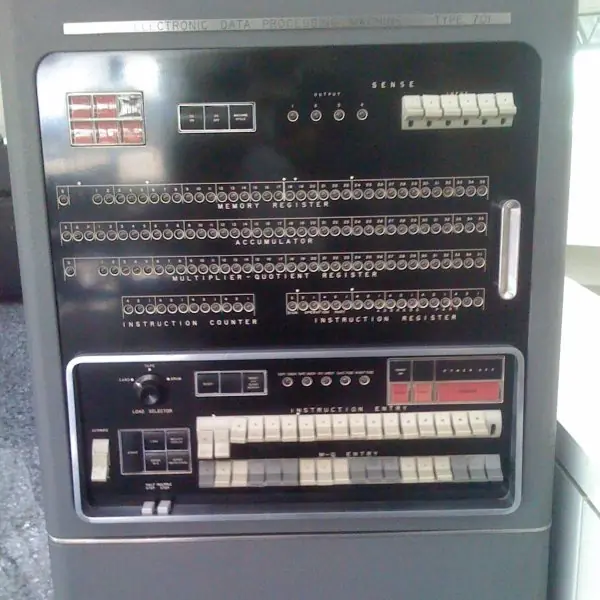
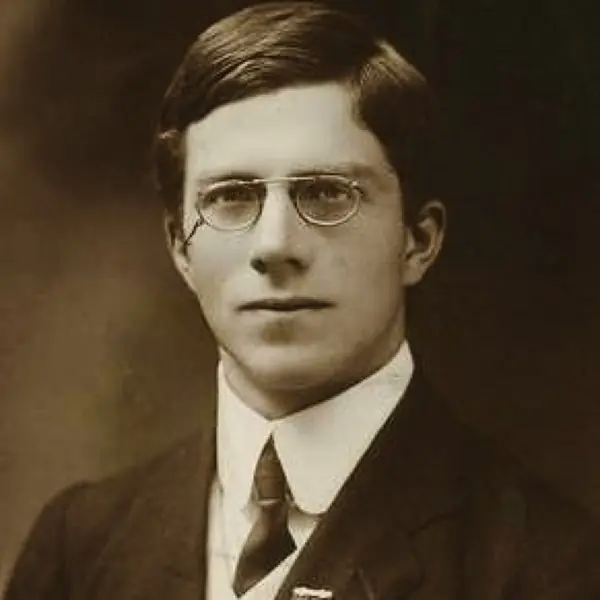
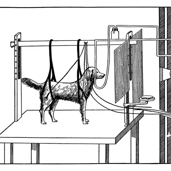
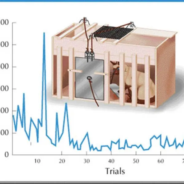
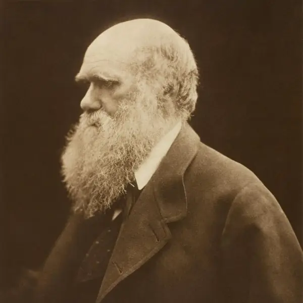
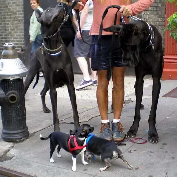
Machine learning is easiest to remember when each algorithm is tied to a picture and to numbers you can check. Plate 4.1 shows the people and machines behind learning from experience.
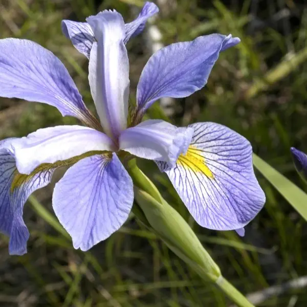
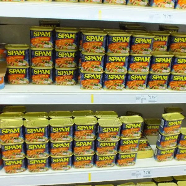
Plate 4.2 shows the three iris flowers of the most famous data set in the field. Plate 4.3 gives an everyday object for spam, clustering and the Overcast branch of the tennis tree.
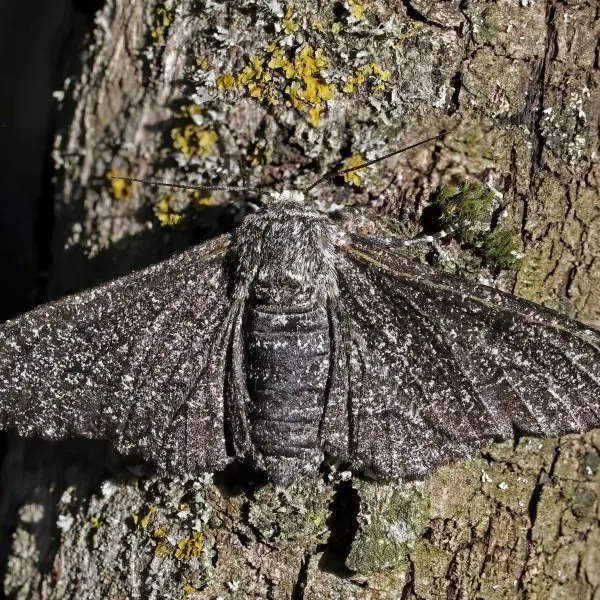
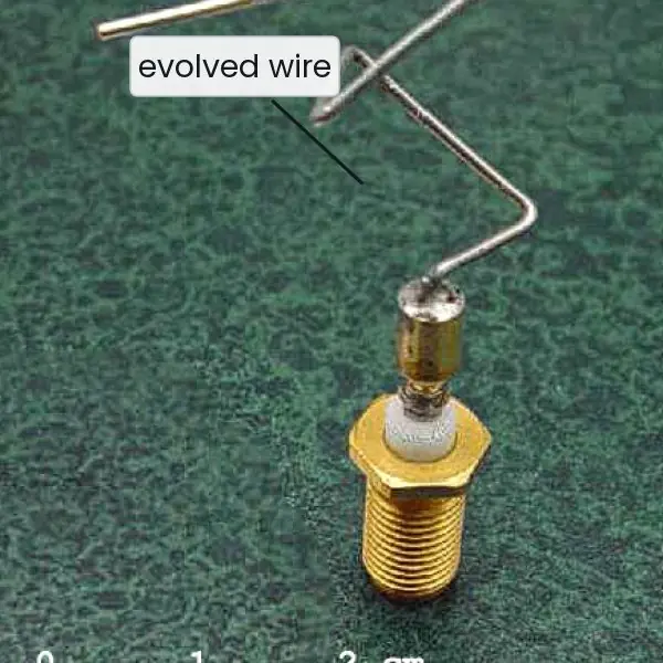
Plate 4.4 collects the natural and engineered examples behind genetic algorithms. The figures after the plates are computed in the figure code itself, so every number printed in a caption is the number the program produced.












4.8.1 Eight uses of machine learning in Nepal
- Spam and scam message filters. Mobile companies such as Nepal Telecom and Ncell, and mail services, must stop unwanted offers and phishing links reaching users. A naive Bayes filter learns from messages that users mark as spam and multiplies the evidence of each word, as in Fig. 4.7. Laplace smoothing keeps a new word from forcing the score to zero. The filter needs regular retraining because scammers change their wording.
- Fraud detection in digital payments. Wallets and banks such as eSewa, Khalti, Fonepay and ConnectIPS see very few fraudulent payments among millions of honest ones. As Fig. 4.4 shows, accuracy is a poor measure here, so the team watches recall (frauds caught) and precision (alarms that were real). A model is trained on past labelled cases and a human checks the alarms that are raised. Too many false alarms would block honest customers.
- Credit scoring for loans. Banks and cooperatives decide on a loan using age, income, savings and repayment history. A decision tree (Fig. 4.6) is popular because the officer can read the path from the first question to the decision and explain it to the customer. The tree must be pruned and tested on new applicants so that it does not overfit (Fig. 4.3). The result supports the officer and does not replace judgement.
- Crop disease and yield prediction. The Department of Agriculture and farm projects hold records of weather, soil, seed and past yields. A k-nearest-neighbour or tree model compares a new field with the most similar earlier fields, as in Fig. 4.8, and suggests a likely yield or a disease risk. Features such as rainfall and altitude must be scaled so that one does not dominate. A farmer should be told when the new field is unlike any earlier one.
- Rain and flood forecasting. The Department of Hydrology and Meteorology records rainfall and river levels at many stations. A regression model learns the relation between upstream rain and later river height, and a classifier learns when a flood warning is needed. The model is tested on seasons it has not seen, because a model that fits only the past years has overfitted. Warnings should always be checked by a forecaster.
- Student progress and dropout alerts. Schools and campuses that record attendance, marks and fees in systems such as Tribhuvan University and school EMIS records can train a tree to flag students at risk of dropping out. Its purpose is to let a teacher offer help early, not to label a child. The data must be checked for bias, for example against students from remote districts, and parents should know how the data is used.
- Customer groups for shops and telecom. A retailer or a mobile company has thousands of customers and no labels for them. k-means groups customers by how much they spend, call or browse, as in Fig. 4.9, and each group gets a suitable offer, such as a data pack for heavy users. The number of groups k and the starting centres matter, so the analyst runs the method several times and keeps the lowest SSE.
- Timetables and delivery routes. A college has to place hundreds of classes in rooms and periods without clashes, and a delivery firm has to plan routes through crowded streets. These are huge search problems with no simple formula. A genetic algorithm, as in Fig. 4.10, evolves many candidate plans, keeps the fit ones and mixes them by crossover. It gives a good plan quickly, though not a guaranteed best one.
Formula and fact sheet
- Entropy H(S) = −Σ pᵢ log₂ pᵢ. Gain(S, A) = H(S) − Σ (|S_v| / |S|) H(S_v). ID3 picks the attribute with the highest gain.
- Naive Bayes: choose C maximising P(C) Π P(xᵢ | C); Laplace: (count + 1) / (n_C + |values|).
- Accuracy, precision = TP/(TP + FP), recall = TP/(TP + FN), F1 = 2PR/(P + R).
- k-NN: majority of the k nearest by distance; scale features.
- GA: selection, crossover, mutation, replacement.
Chapter summary
- Machine learning improves a task from data: supervised (labelled), unsupervised (structure), reinforcement (rewards); evaluate on unseen data to detect overfitting.
- Rote learning memorises, analogy reuses similar cases, induction generalises, explanation-based learning generalises from one explained example.
- Decision trees split on the attribute with the highest information gain; naive Bayes multiplies class-conditional probabilities; k-NN votes among nearest neighbours.
- Genetic algorithms evolve a population with selection, crossover and mutation.
Practice
- Differentiate supervised, unsupervised and reinforcement learning with an example each.
- What is overfitting and how can it be reduced?
- Compute accuracy, precision, recall and F1 for TP = 40, FP = 10, FN = 20, TN = 130.
- Explain rote learning, learning by analogy and explanation-based learning.
- Compute the entropy of a set with 9 positive and 5 negative examples.
- Why does ID3 choose Outlook as the root of PlayTennis? Give the gains.
- Classify (Sunny, Cool, High, Strong) with naive Bayes and give the probabilities.
- What is the zero-frequency problem and how does Laplace smoothing fix it?
- Classify q = (3, 3) with 1-NN for the data in Section 4.5.
- Describe the steps of a genetic algorithm and perform single-point crossover on 11100011 and 00011110 after bit 5.
Answers and worked solutions
1. Supervised: spam classification from labelled mail. Unsupervised: grouping customers by purchases. Reinforcement: a robot learning to walk from rewards.
2. The model fits noise in the training data and generalises poorly. Reduce it with more data, simpler models, pruning or regularisation, and cross-validation to detect it.
3. Accuracy 0.85; precision 40/50 = 0.80; recall 40/60 = 0.667; F1 = 2 × 0.8 × 0.667 / (0.8 + 0.667) = 0.727.
4. Rote: store and recall answers. Analogy: adapt the solution of the most similar earlier case. EBL: explain why one example works using domain knowledge and generalise the explanation.
5. H = −(9/14) log₂(9/14) − (5/14) log₂(5/14) = 0.940 bits.
6. Gain(Outlook) = 0.247 is larger than Humidity 0.152, Wind 0.048 and Temperature 0.029.
7. Score(Yes) = 0.0053, Score(No) = 0.0206; P(No) = 0.795, P(Yes) = 0.205; the class is No.
8. An unseen value gives probability 0 and forces the whole product to 0; add-one smoothing gives it a small non-zero probability, (count + 1)/(n + |values|).
9. The nearest point is (4, 4) at distance 1.414, class B.
10. Initialise, evaluate fitness, select parents, crossover, mutate, replace, repeat. Crossover after bit 5: 11100|011 and 00011|110 give 11100110 and 00011011.
Model answers for Unit 4
Q1. Define machine learning. Explain supervised, unsupervised and reinforcement learning with examples. (10 marks)
Introduction. Machine learning is the study of programs that improve at a task through experience.
In Mitchell's wording, a program learns from experience E with respect to a task T and a performance measure P if its performance at T, measured by P, improves with E. A spam filter has the task of classifying mail, the measure of accuracy and the experience of mails that users have labelled.
Kinds of learning (Fig. 4.1).
- Supervised learning uses training data that has inputs and the correct outputs. The program learns the map from input to output. If the output is a category the task is classification (spam or not spam, a digit from 0 to 9); if it is a number the task is regression (the price of a house). Decision trees, naive Bayes, k-nearest neighbours and neural networks are examples.
- Unsupervised learning has no labels. The program finds structure by itself: clustering groups similar customers, association rules find that buyers of tea also buy sugar, and dimensionality reduction compresses many features into few. k-means is the standard example.
- Reinforcement learning places an agent in a world. It acts, receives a reward or a penalty, and learns by trial and error which actions give the largest total reward. Game players and robots that learn to walk are examples, and Thorndike's puzzle box in Plate 4.1 is the animal version.
- Semi-supervised learning uses a few labelled examples and many unlabelled ones, which is useful when labelling is expensive.
| Point | Supervised | Unsupervised | Reinforcement |
|---|---|---|---|
| Data | inputs and labels | inputs only | states, actions, rewards |
| Goal | predict the label | find structure | maximise total reward |
| Feedback | correct answer | none | reward after actions |
| Example | spam filter | customer groups | game player |
Evaluation. Whatever the kind, the data is split into training, validation and test sets, and the final score is measured on the test set. A model that does well only on the training data has overfitted (Fig. 4.3).
Conclusion. The three kinds differ in the feedback they receive: the right answer, no answer, or a reward. The choice of method follows from what data is available (Fig. 4.11).
Q2. What is overfitting? How can it be detected and reduced? (5 marks)
A model overfits when it fits the training data very closely, including its random noise, and then performs badly on new data. It has memorised instead of generalising. The opposite fault is underfitting, where the model is too simple to capture the pattern.
Evidence (Fig. 4.3). Twelve noisy points from a sine curve were fitted with polynomials of degree 1 to 10. The training error fell steadily from 0.362 to 0.042, which looks like steady improvement.
On 60 new points, however, the error was smallest at degree 3 (0.311) and then grew to 1.107 at degree 5 and 998.9 at degree 10. Degree 1 underfits (0.494) and degree 10 overfits.
Detection. Keep a test set that the model never sees during training; a large gap between training and test accuracy signals overfitting.
Cross-validation divides the data into k folds and uses each fold once as the test set, so the estimate does not depend on one lucky split.
Reduction.
- Collect more training data.
- Choose a simpler model (lower degree, fewer attributes).
- Prune a decision tree, or limit its depth.
- Use regularisation, which penalises large weights.
- Stop training early when the validation error starts to rise.
Conclusion. The aim of learning is good performance on unseen cases, so the model is judged on the test set and not on the training set.
Q3. Define accuracy, precision, recall and F1. Compute them for TP = 40, FP = 10, FN = 20, TN = 130 and explain why accuracy can mislead. (5 marks)
For a two-class problem count the true positives (TP), false positives (FP), false negatives (FN) and true negatives (TN), as in the confusion matrix of Fig. 4.4.
| Measure | Formula | Meaning |
|---|---|---|
| Accuracy | (TP + TN) / total | fraction of all cases correct |
| Precision | TP / (TP + FP) | of those called positive, how many are positive |
| Recall | TP / (TP + FN) | of the real positives, how many were found |
| F1 | 2PR / (P + R) | harmonic mean of precision and recall |
Computation. The total is 40 + 10 + 20 + 130 = 200. Accuracy = (40 + 130) / 200 = 0.85. Precision = 40 / 50 = 0.80. Recall = 40 / 60 = 0.667. F1 = 2 × 0.80 × 0.667 / (0.80 + 0.667) = 0.727.
Why accuracy misleads. Suppose 10 of 10,000 payments are fraudulent. A model that always says not fraud is right 9,990 times, an accuracy of 99.90 percent, and catches no fraud at all.
A real detector with 8 true positives and 40 false positives has a lower accuracy of 99.58 percent but a recall of 0.80. When classes are rare, precision, recall and F1 describe the usefulness of the model better than accuracy.
Q4. Explain the ID3 decision-tree algorithm. Build the tree for the PlayTennis data using entropy and information gain. (10 marks)
Introduction. A decision tree classifies a case by asking a series of questions. Each internal node tests an attribute, each branch is one value of it and each leaf gives a class.
ID3 builds the tree greedily from the top, choosing at every node the attribute with the largest information gain.
Measures. Entropy measures impurity: H(S) = −Σ pᵢ log₂ pᵢ, which is 0 for a pure set and 1 bit for a 50/50 mix. The information gain of an attribute A is Gain(S, A) = H(S) − Σ (|S_v| / |S|) H(S_v), the drop in entropy after splitting on A (Fig. 4.5).
Algorithm.
- If all examples at the node have the same class, make a leaf.
- If there are no attributes left, make a leaf with the majority class.
- Otherwise compute the gain of each remaining attribute and split on the best one.
- Repeat for each branch with the examples that have that value.
Worked example. The 14 days have 9 Yes and 5 No, so H(S) = 0.940. The gains are Outlook 0.247, Humidity 0.152, Wind 0.048 and Temperature 0.029, so Outlook is the root. The Overcast branch has 4 Yes and no No, so it is a leaf (Yes).
The Sunny branch (2 Yes, 3 No) has its best split on Humidity (High gives No, Normal gives Yes). The Rain branch (3 Yes, 2 No) is best split on Wind (Weak gives Yes, Strong gives No). Fig. 4.6 shows the tree.
The day Sunny, Cool, High, Strong is classified No.
| Point | Decision tree |
|---|---|
| Strength | easy to read and explain; handles mixed data |
| Weakness | overfits; small data changes alter the tree |
| Remedy | pruning, or a random forest of many trees |
| Variants | C4.5 (gain ratio, continuous values), CART (Gini index) |
Conclusion. ID3 builds a short, readable tree by always taking the most informative question first. The tree should be pruned and tested on unseen data before it is trusted.
Q5. Explain the naive Bayes classifier. Classify (Sunny, Cool, High, Strong) for PlayTennis and explain Laplace smoothing. (10 marks)
Introduction. Naive Bayes applies Bayes' rule with the assumption that, given the class, the attributes are independent. It chooses the class C that maximises P(C) × Π P(xᵢ | C).
The assumption is rarely exactly true, but the method is fast, needs little data and works well for text.
Priors and likelihoods. From the 14 days, P(Yes) = 9/14 and P(No) = 5/14. The likelihoods are given in Fig. 4.7:
| Evidence | P(· | Yes) | P(· | No) |
|---|---|---|
| Outlook = Sunny | 2/9 | 3/5 |
| Temperature = Cool | 3/9 | 1/5 |
| Humidity = High | 3/9 | 4/5 |
| Wind = Strong | 3/9 | 3/5 |
Scores. Score(Yes) = 9/14 × 2/9 × 3/9 × 3/9 × 3/9 = 0.0053. Score(No) = 5/14 × 3/5 × 1/5 × 4/5 × 3/5 = 0.0206. Dividing by the sum, P(No) = 0.0206 / 0.0259 = 0.795 and P(Yes) = 0.205. The prediction is No: do not play.
The zero-frequency problem. If a value never occurred with a class in training, its estimated probability is 0 and the whole product becomes 0, however strong the other evidence.
Laplace (add-one) smoothing estimates P(word | class) = (count + 1) / (words in class + V), where V is the number of distinct words.
In the spam example with V = 11, the message cheap pills gets a spam score of 0.0148 and a ham score of 0.0015, so P(spam) = 0.908. Without smoothing the ham score would be 0 whatever the words were.
Strengths and limits. Naive Bayes trains in one pass over the data, so it is fast even for large text collections, and it gives a probability and not only a label.
Its independence assumption is false when attributes are linked, for example the words New and Kathmandu, which can make the probabilities too extreme, although the ranking of classes is often still right.
It should therefore be tested on unseen data like any other model.
Conclusion. Naive Bayes multiplies the evidence for each class and picks the larger score. Laplace smoothing is essential for text, where new words appear all the time.
Q6. Describe the k-nearest-neighbour method. How is k chosen and why are features scaled? (5 marks)
k-NN is a lazy, instance-based learner. It has no training phase: it stores all the examples and does its work when a query arrives.
To classify a query it finds the k training points closest to it, usually by Euclidean distance, and takes a majority vote of their classes. For regression it averages their values.
Example (Fig. 4.8). On 30 real iris flowers the query (4.8, 1.6) has five nearest neighbours at distances 0.141, 0.141, 0.224, 0.224 and 0.424. Three are versicolor and two are virginica, so the answer is versicolor.
In the toy example of Section 4.5 the point (3, 3) has nearest neighbour (4, 4) at distance 1.414, class B.
Choosing k. A small k gives a noisy boundary that follows single odd points; a large k blurs the classes together.
For the 30 flowers the leave-one-out accuracy is 28/30 at k = 1, 29/30 at k = 3, 28/30 at k = 5, 29/30 at k = 7 and 26/30 at k = 9. So k is chosen by validation, and an odd k avoids ties in a two-class problem.
Scaling. Distance adds the differences of all features. If income is in rupees and age in years, the income difference swamps the age difference, so every feature is first scaled to a similar range, for example to 0 to 1.
Conclusion. k-NN is simple and needs no model, but it is slow for large data and sensitive to scaling and to irrelevant features.
Q7. Explain the k-means clustering algorithm. What are its weaknesses? (5 marks)
Clustering is unsupervised: it groups similar points without labels. k-means groups n points into k clusters.
Algorithm.
- Choose k starting centres (random points, for example).
- Assign every point to its nearest centre.
- Update each centre to the mean of the points assigned to it.
- Repeat steps 2 and 3 until no assignment changes.
The method minimises the sum of squared distances (SSE) of points to their own centre. SSE never rises from one round to the next, so the loop must stop.
Example (Fig. 4.9). On 30 iris flowers with k = 3 and one starting centre in each group, the SSE falls 17.3, 7.2, 7.1 and the loop stops after 3 rounds; the clusters follow the three species.
With all three starting centres inside the setosa group the SSE ends at 20.43, almost three times worse.
Weaknesses.
- The result depends on the starting centres, so the method is run several times and the lowest SSE is kept.
- k must be chosen in advance.
- It finds round clusters of similar size and is disturbed by outliers.
- Features need scaling.
Conclusion. k-means is fast and simple, but its answer is only a local minimum and must be checked.
Q8. Explain the genetic algorithm with its steps. Show one generation of an example. (10 marks)
Introduction. A genetic algorithm (GA) is a search method that copies natural selection (Plate 4.4).
It keeps a population of candidate solutions, each written as a chromosome such as a bit string, and improves the population over generations. It suits hard optimisation problems where the landscape is badly understood.
Steps.
- Initialise a random population.
- Evaluate the fitness of each individual with a fitness function.
- Select parents with a chance that grows with fitness (roulette wheel or tournament).
- Crossover: choose a cut point and swap the tails of two parents to make children.
- Mutation: flip each bit with a small probability, which keeps variety in the population.
- Replace the population (often keeping the best individual, called elitism) and repeat until the fitness is good enough or time runs out.
Worked example (Fig. 4.10). Maximise f(x) = x² for x from 0 to 31 with 5-bit strings. The population 01101, 11000, 01000 and 10011 has x values 13, 24, 8 and 19, fitness 169, 576, 64 and 361, a total of 1170 and a mean of 292.5.
The roulette shares are 14.4, 49.2, 5.5 and 30.9 percent, so 11000 is most likely to be chosen. Crossing 11000 with 10011 after bit 2 gives 11011 (x = 27, fitness 729) and 10000 (fitness 256).
A child of 729 is already better than any parent.
A real run. On 30-bit strings the best fitness rose from 19 to the maximum of 30 in generation 15 (about 480 evaluations).
| Point | Genetic algorithm |
|---|---|
| Strength | needs no gradient; handles huge, rough search spaces |
| Weakness | many fitness evaluations; no guarantee of the best answer |
| Sensitivity | depends on the encoding, population size and mutation rate |
| Uses | timetables, routes, circuit and antenna design |
Conclusion. A GA improves a population by selection, crossover and mutation. It gives good solutions to problems that are too large to search completely, such as the evolved antenna of Plate 4.4.
Q9. Explain rote learning, learning by analogy, inductive learning and explanation-based learning. (5 marks)
Fig. 4.2 summarises the four forms.
- Rote learning stores every input and output pair and looks the answer up later. Samuel's checkers program stored the values of positions it had met, and a web cache stores pages. It gives speed but no ability to handle a new case.
- Learning by analogy (case-based reasoning) solves a new problem by finding the most similar earlier case and adapting its solution. A help desk retrieves the nearest earlier fault and adjusts its fix. The k-NN method is a simple form, and the quality of the similarity measure decides the quality of the answer.
- Inductive learning generalises from many examples to a rule that covers unseen cases, such as learning the rule for a bird from many labelled animals. Induction is never certain, because one new case can break the rule, and many rules fit the same data, so a bias such as Occam's razor (prefer the simpler rule) is needed. Decision trees and neural networks are inductive.
- Explanation-based learning (EBL) uses background knowledge to explain why one example works, then generalises the explanation into a macro-rule. One example may be enough, but a correct domain theory is required.
Conclusion. The four forms differ in how much they generalise: rote none, analogy a little, induction a lot from many examples, and EBL a lot from one example plus knowledge.