Unit 2 · Microeconomics · 30 teaching hours · 47 min read
Microeconomics (व्यष्टि अर्थशास्त्र)
What the syllabus asks for 7
- Revenue: total, average and marginal revenue and their curves under perfect competition and monopoly
- Demand and supply: law, determinants, elasticity; market equilibrium
- Cost: fixed, variable, total, average and marginal cost and their curves
- Production: factors of production, law of variable proportions, returns to scale
- Market structures: perfect competition, monopoly, monopolistic competition and oligopoly
- Price and output determination under perfect competition and monopoly
- Distribution: rent, wages, interest and profit; marginal productivity theory of distribution
Microeconomics is the study of the individual decision — one consumer choosing how much to buy, one firm choosing how much to produce, one market settling on a price. The whole unit turns on two pairs of curves.
The first pair is revenue — what a firm takes in — and cost — what it gives out; the difference between them is profit, and the firm's whole purpose is to make that difference as large as it can.
The second pair is demand and supply, which together fix the price at which every one of those decisions is taken.
This unit builds the two pairs from the ground up, uses them to explain how price and output are determined under different market structures, and ends with how the price of the factors of production themselves is decided.
This unit carries the largest share of the paper — 30 of the 96 teaching hours and a corresponding share of the marks.
Group B almost always gives a table of price and quantity and asks you to fill in TR, AR and MR, or asks for the features of perfect competition or monopoly, or the relation between AC and MC.
Group C may ask for price and output determination under perfect competition or monopoly, or for the law of variable proportions, or for the marginal productivity theory of distribution.
Practise the tables until you can fill them without thinking: TR = P × Q, AR = TR ÷ Q, MR = change in TR ÷ change in Q.
2.1 Revenue and revenue curves
A firm's revenue is the money it receives from selling its output. Three measures matter.
| Measure | Definition | Formula |
|---|---|---|
| Total revenue (TR) | The whole amount received from the sale of a given quantity | TR = Price \times Quantity |
| Average revenue (AR) | Revenue per unit sold — which is simply the price of the good | AR = \frac{TR}{Q} |
| Marginal revenue (MR) | The addition to total revenue from selling one more unit | MR = \frac{\Delta TR}{\Delta Q} |
The relations that must be learned:
- When MR is positive, TR is rising; when MR is zero, TR is at its maximum; when MR is negative, TR is falling.
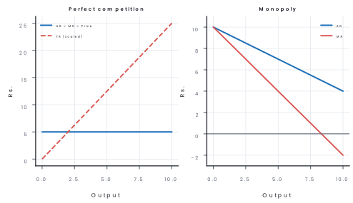
- When price is constant (that is, under perfect competition), AR = MR = Price, and TR rises as a straight line.
- When price must be lowered to sell more (that is, under monopoly and monopolistic competition), AR falls, MR falls twice as fast as AR, and TR rises at a decreasing rate and then falls.
Perfect competition. The firm is so small a part of the market that it can sell any quantity at the market price. Price is therefore fixed for the firm, and AR, MR and price are all the same and constant.
All three are drawn as one horizontal straight line. TR is a straight line through the origin whose slope is the price.
Monopoly. The firm is the whole market, so to sell more it must lower the price for all the units it sells, not only the extra one. As a result AR slopes downwards, and MR lies below AR and falls twice as steeply.
TR rises while MR is positive, is maximum where MR cuts the quantity axis, and falls after that.
Problem. The following table gives the price at which different quantities of a commodity can be sold. Complete the table by finding the total revenue, the average revenue and the marginal revenue.
| Price (Rs.) | Quantity sold | TR | AR | MR |
|---|---|---|---|---|
| 12 | 0 | … | … | … |
| 10 | 1 | … | … | … |
| 9 | 2 | … | … | … |
| 8 | 3 | … | … | … |
| 7 | 4 | … | … | … |
| 6 | 5 | … | … | … |
| 5 | 6 | … | … | … |
| 4 | 7 | … | … | … |
Solution. Step 1 — TR = Price \times Quantity. Step 2 — AR = \frac{TR}{Q}, which must equal the price. Step 3 — MR = TR of this row − TR of the previous row.
| Price (Rs.) | Quantity | TR (Rs.) | AR (Rs.) | MR (Rs.) |
|---|---|---|---|---|
| 12 | 0 | 0 | — | — |
| 10 | 1 | 10 | 10 | 10 |
| 9 | 2 | 18 | 9 | 8 |
| 8 | 3 | 24 | 8 | 6 |
| 7 | 4 | 28 | 7 | 4 |
| 6 | 5 | 30 | 6 | 2 |
| 5 | 6 | 30 | 5 | 0 |
| 4 | 7 | 28 | 4 | −2 |
Answer. As in the table. What it means. Three things are worth noticing. AR always equals the price. MR falls faster than AR, because the price cut also applies to the units that could have been sold at the old price.
And TR reaches its maximum of Rs. 30 at 5 to 6 units and then falls, exactly where MR passes through zero and turns negative.
2.2 Demand and supply
Demand (माग) is the quantity of a good that consumers are willing and able to buy at a given price in a given period. It is not the same as desire: a wish without the money to buy it is not demand.
The law of demand. Other things remaining the same, when the price of a good rises, the quantity demanded falls; when the price falls, the quantity demanded rises. So the demand curve slopes downwards from left to right.
Why? Three reasons. The income effect: a fall in price leaves the consumer with more real income, so he buys more. The substitution effect: when the price of one good falls relative to others, consumers substitute it for the others.
The law of diminishing marginal utility: as a consumer has more of a good, each further unit gives him less satisfaction, so he will buy more only at a lower price.
Determinants of demand other than price. Income; the prices of related goods (substitutes and complements); tastes and fashion; expectations of future prices; the size and structure of the population; the distribution of income; and the season.
Movement along and shift of the demand curve. A change in the price of the good itself causes a movement along the curve (an extension or a contraction of demand).
A change in any other determinant shifts the whole curve to a new position — a shift (increase or decrease) of demand.
Supply (पूर्ति) is the quantity of a good that producers are willing and able to offer for sale at a given price in a given period.
The law of supply. Other things remaining the same, when the price rises, the quantity supplied rises, and when the price falls, the quantity supplied falls. The supply curve therefore slopes upwards, because a higher price covers the higher cost of producing more, and attracts new producers into the market.
Elasticity of demand. The price elasticity of demand measures how strongly the quantity demanded responds to a change in price.
| Value of E_d | Name | Meaning |
|---|---|---|
| E_d = 0 | Perfectly inelastic | Quantity does not change at all with price |
| E_d < 1 | Relatively inelastic | Quantity changes proportionately less than price — salt, medicine |
| E_d = 1 | Unitary elastic | Quantity changes in the same proportion as price |
| E_d > 1 | Relatively elastic | Quantity changes proportionately more than price — luxury goods |
| E_d = \infty | Perfectly elastic | Any quantity is bought at one price |
Market equilibrium. Where the demand curve and the supply curve cross, the quantity demanded equals the quantity supplied. That price is the equilibrium price and that quantity the equilibrium quantity.
If the price is above equilibrium, supply exceeds demand and unsold stock pushes the price down; if it is below equilibrium, demand exceeds supply and competition among buyers pushes the price up.
This is what Adam Smith called the invisible hand: no one orders the market, and yet it settles.
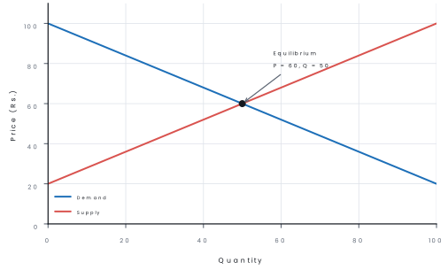
Problem.(a) When the price of a commodity falls from Rs. 10 to Rs. 8, the quantity demanded rises from 40 units to 50 units. Find the price elasticity of demand and say whether the demand is elastic or inelastic.(b) In a market, Q_d = 100 - 2P and Q_s = 20 + 2P. Find the equilibrium price and the equilibrium quantity.
Solution. Step 1 —(a) Change in quantity = 50 - 40 = 10 units; percentage change = \frac{10}{40} \times 100 = 25\%. Step 2 — Change in price = 8 - 10 = -2; percentage change = \frac{-2}{10} \times 100 = -20\%. Step 3 — E_d = \frac{25\%}{-20\%} = -1.25. Taking the absolute value, E_d = 1.25. Step 4 — Since E_d > 1, the demand is relatively elastic. Step 5 —(b) At equilibrium Q_d = Q_s: 100 - 2P = 20 + 2P. Step 6 — 80 = 4P, so P = Rs.\ 20. Step 7 — Q = 100 - 2(20) = 60 units. Check with supply: 20 + 2(20) = 60. ✔
Answer.(a) E_d = 1.25 — elastic.(b) Equilibrium price Rs. 20, equilibrium quantity 60 units. What it means. An elasticity above one tells a seller something valuable: cutting the price raises total revenue, because the quantity sold rises by proportionately more than the price falls. Below one, the reverse is true. And at Rs. 20, no buyer wants to offer more and no seller wants to ask less, so the price stays.
2.3 Cost and cost curves
Cost of production is the total money expense a firm has to bear in producing a given quantity of output. It is divided first into fixed and variable cost.
| Concept | Short name | Meaning | Formula |
|---|---|---|---|
| Total fixed cost | TFC | Cost that does not change with output — rent, insurance, the salary of permanent staff | Constant |
| Total variable cost | TVC | Cost that changes directly with output — raw materials, wages of casual labour, power | Varies with Q |
| Total cost | TC | The whole cost of producing the output | TC = TFC + TVC |
| Average fixed cost | AFC | Fixed cost per unit | AFC = \frac{TFC}{Q} |
| Average variable cost | AVC | Variable cost per unit | AVC = \frac{TVC}{Q} |
| Average total cost | ATC (or AC) | Total cost per unit | ATC = \frac{TC}{Q} = AFC + AVC |
| Marginal cost | MC | The addition to total cost from producing one more unit | MC = \frac{\Delta TC}{\Delta Q} |
The shapes, and why. TFC is a horizontal straight line. TVC rises as output rises and, beyond a point, rises faster, because of diminishing returns. TC has the same shape as TVC but starts above the origin by the amount of TFC.
AFC falls continuously as output rises and approaches zero but never reaches it — fixed cost is spread thinner and thinner.
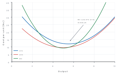
AVC, ATC and MC are all U-shaped: they fall at first as the fixed and then the variable inputs are used better, reach a minimum, and then rise as diminishing returns set in.
The relations that examiners test.
- MC cuts AVC and ATC at their minimum points. This is the most asked relation in the whole chapter. While MC is below AC, AC is falling; while MC is above AC, AC is rising; so MC must pass through AC exactly at AC's lowest point.
- AFC is the vertical distance between ATC and AVC, and it shrinks as output grows, so ATC and AVC come closer together.
- MC is the change in TC, and also the change in TVC, because TFC does not change: MC = \frac{\Delta TC}{\Delta Q} = \frac{\Delta TVC}{\Delta Q}.
- The AC curve is U-shaped because the fall in AFC and the initial fall in AVC outweigh the later rise in AVC, and then the rise in AVC outweighs the continuing fall in AFC.
Problem. A firm's total fixed cost is Rs. 60 and its total variable cost at different outputs is as given. Complete the table.
| Q | TFC | TVC | TC | AFC | AVC | ATC | MC |
|---|---|---|---|---|---|---|---|
| 0 | 60 | 0 | … | … | … | … | … |
| 1 | 60 | 40 | … | … | … | … | … |
| 2 | 60 | 70 | … | … | … | … | … |
| 3 | 60 | 96 | … | … | … | … | … |
| 4 | 60 | 130 | … | … | … | … | … |
| 5 | 60 | 180 | … | … | … | … | … |
| 6 | 60 | 252 | … | … | … | … | … |
Solution. Step 1 — TC = TFC + TVC. Step 2 — AFC = \frac{TFC}{Q}, AVC = \frac{TVC}{Q}, ATC = \frac{TC}{Q}. Step 3 — MC = TC of this row − TC of the previous row.
| Q | TFC | TVC | TC | AFC | AVC | ATC | MC |
|---|---|---|---|---|---|---|---|
| 0 | 60 | 0 | 60 | — | — | — | — |
| 1 | 60 | 40 | 100 | 60.00 | 40.00 | 100.00 | 40 |
| 2 | 60 | 70 | 130 | 30.00 | 35.00 | 65.00 | 30 |
| 3 | 60 | 96 | 156 | 20.00 | 32.00 | 52.00 | 26 |
| 4 | 60 | 130 | 190 | 15.00 | 32.50 | 47.50 | 34 |
| 5 | 60 | 180 | 240 | 12.00 | 36.00 | 48.00 | 50 |
| 6 | 60 | 252 | 312 | 10.00 | 42.00 | 52.00 | 72 |
Answer. As in the table. What it means. AFC falls throughout, from Rs. 60 to Rs. 10. ATC falls to a minimum of Rs. 47.50 at 4 units and then rises.
MC is lowest (Rs. 26) at 3 units, before ATC reaches its minimum — and it cuts ATC between 4 and 5 units, exactly where ATC turns up. That is the relation the examiner wants you to see.
2.4 Production: factors, the law of variable proportions and returns to scale
Production is the creation of goods and services that satisfy human wants. The factors of production — land, labour, capital and entrepreneurship — are combined in a certain proportion to produce output.
The proportion in which they are combined is the technique of production: labour-intensive if labour is used heavily (a rickshaw puller, hand-looms, terrace farming) and capital-intensive if machinery is used heavily (a hydropower plant, a cement factory).
The law of variable proportions (returns to a variable factor). This is the short-run law, in which at least one factor is fixed — usually capital, say a fixed factory — and the other, labour, is varied.
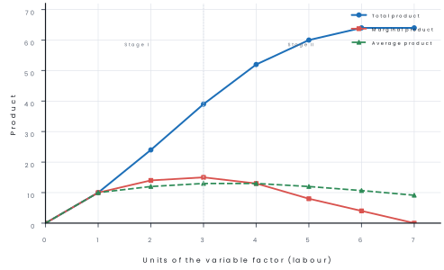
As more and more units of a variable factor are applied to a fixed factor, total product first increases at an increasing rate, then increases at a diminishing rate, and finally declines.
The three stages.
| Stage | Total product | Marginal product | Average product | What is happening |
|---|---|---|---|---|
| I — Increasing returns | Rises at an increasing rate | Rises, then reaches its maximum | Rises, but is below MP | The fixed factor is under-used; adding labour lets it be used better and allows specialisation |
| II — Diminishing returns | Rises, but at a diminishing rate | Falls, but stays positive | Rises to a maximum, then falls; MP cuts AP at AP's maximum | The fixed factor is now fully used; each extra worker has less of it to work with |
| III — Negative returns | Falls | Negative | Falls | There are so many workers that they get in one another's way |
Why MP cuts AP at AP's maximum. While MP is above AP, AP is being pulled up; while MP is below AP, AP is pulled down; so MP must cross AP exactly where AP is at its highest.
This is the same reasoning as MC cutting AC, and the two are the pair of relations most often asked.

Returns to scale is a long-run idea: here all the factors are varied together, and the firm's scale itself changes.
- Increasing returns to scale — output rises by a larger proportion than the inputs (doubling all inputs more than doubles output). Causes: specialisation and division of labour, indivisibility of machines, and the use of by-products.
- Constant returns to scale — output rises in exactly the same proportion as the inputs.
- Decreasing returns to scale — output rises by a smaller proportion than the inputs. Causes: the difficulty of managing a very large organisation, rising marketing and transport costs, and the exhaustion of natural resources.
The distinction matters: the law of variable proportions is a short-run law with one factor fixed; returns to scale is a long-run law with all factors variable.
Problem. With a fixed factory of one hectare, the total product of labour is as follows.
| Labour | 0 | 1 | 2 | 3 | 4 | 5 | 6 | 7 |
|---|---|---|---|---|---|---|---|---|
| Total product (quintals) | 0 | 10 | 24 | 39 | 52 | 60 | 64 | 64 |
Find the marginal product and the average product, and state in which units of labour each of the three stages of the law of variable proportions operates.
Solution. Step 1 — MP = TP of this row − TP of the previous row. Step 2 — AP = \frac{TP}{L}.
| Labour | TP | MP | AP | Stage |
|---|---|---|---|---|
| 1 | 10 | 10 | 10 | I — increasing |
| 2 | 24 | 14 | 12 | I — increasing |
| 3 | 39 | 15 | 13 | I ends here (MP is at its maximum) |
| 4 | 52 | 13 | 13 | II — diminishing (AP = MP at AP's maximum) |
| 5 | 60 | 8 | 12 | II — diminishing |
| 6 | 64 | 4 | 10.67 | II — diminishing |
| 7 | 64 | 0 | 9.14 | II ends here (MP = 0, TP is maximum) |
Step 3 — Stage I runs up to the 3rd worker (MP still rising). Stage II runs from the 4th to the 6th (MP falling but positive, TP still rising). A 7th worker adds nothing (MP = 0); an 8th would make MP negative and TP would fall — that is Stage III.
Answer. Stage I: 1st to 3rd worker. Stage II: 4th to 6th. Stage III: from the 8th worker onwards. What it means. The farmer should employ between 4 and 6 workers — the point where marginal product is positive.
Note that AP is maximum at the 4th worker, exactly where MP equals AP, which is the boundary between the first two stages.

2.5 Market structures
A market in economics is not a place but the whole set of buyers and sellers of a good, together with the terms on which they deal.
A market structure describes how many firms there are, what kind of product they sell, whether they can enter and leave freely, and how much any one of them can influence the price.
| Feature | Perfect competition | Monopoly | Monopolistic competition | Oligopoly |
|---|---|---|---|---|
| Number of sellers | Very many | One | Many | A few |
| Product | Homogeneous (identical) | No close substitute | Differentiated (branded) | Homogeneous or differentiated |
| Entry and exit | Completely free | Blocked | Free | Difficult |
| Price control by a firm | None — a price taker | Considerable — a price maker | Some, within limits | Interdependent; a price war harms all |
| Demand curve faced by the firm | Perfectly elastic (horizontal) | Downward sloping | Downward sloping, fairly elastic | Kinked or uncertain |
| Selling cost (advertising) | None | Some (publicity) | Heavy | Very heavy |
| Example | A vegetable market; wheat | Nepal Telecom in its early years; a patented drug | Soap, tea, restaurants, cloth shops | Mobile network operators, airlines |
Perfect competition is a theoretical model, but a useful one, because it shows the best that a market can do if nothing interferes.
Its features are: a very large number of buyers and sellers, so that no single one can influence the price; a homogeneous product; free entry and exit; perfect knowledge of the market; perfect mobility of the factors of production; and no transport cost.
Monopoly exists when a single firm is the only seller of a good that has no close substitute, and entry is blocked — by a patent, a licence, control of a raw material, or sheer scale.
A natural monopoly arises where the fixed cost is so large that two firms would both lose money, as with a drinking-water or electricity distribution network.
A monopolist is a price maker, but not free to charge anything: the demand curve still limits him, and a price so high that people stop buying earns less than a moderate one.
Monopolistic competition is the commonest real market: many sellers, free entry, but each seller's product is slightly different — by brand, quality, location, packaging or service.
Because the product is differentiated, each firm faces a slightly downward-sloping demand curve and has a little price power; because entry is free, abnormal profit attracts new firms and is competed away in the long run, much of the competition taking the form of advertising rather than price.
Oligopoly is a market with a few large sellers whose decisions are interdependent: each firm must guess what the others will do before it changes its price or its output.
That interdependence explains why oligopolies often prefer non-price competition — advertising, product variation, service — and can settle into price rigidity or into collusion.
2.6 Price and output determination
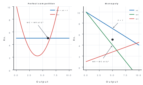
Every firm, whatever its market, maximises profit by producing the output at which marginal cost equals marginal revenue (MC = MR), provided that MC is rising at that point. There are two conditions for equilibrium.
- First order condition: MC = MR — the last unit produced adds exactly as much to cost as to revenue, so no more and no less should be produced.
- Second order condition: MC must be rising (or at least cutting MR from below) at that output, so that the firm is at a maximum and not a minimum of profit.
Under perfect competition. Price is given by the market, so AR = MR = P. The firm's equilibrium is where MC = P.
- If P > ATC, the firm earns abnormal (supernormal) profit.
- If P = ATC, it earns only normal profit — the break-even or shut-down point of the long run.
- If AVC < P < ATC, it makes a loss but continues in the short run, because it covers all its variable cost and part of its fixed cost.
- If P < AVC, it shuts down at once: producing only adds to the loss.
Under monopoly. The firm equates MC with MR, and then reads the price off the AR curve at that output — which is why a monopolist's price is higher than its marginal cost, and higher than the price that would rule under competition.
Output is lower and price is higher than under perfect competition; the monopolist takes a part of the consumer's surplus, which is called the deadweight loss to society.
Problem. A monopolist faces the demand function P = 100 - 2Q, where P is the price in rupees and Q the output in units. The firm's marginal cost is constant at Rs. 20. Find(a) the marginal revenue function,(b) the profit-maximising output,(c) the price charged, and(d) the profit if the average total cost at that output is Rs. 40.
Solution. Step 1 — Total revenue TR = P \times Q = (100 - 2Q)Q = 100Q - 2Q^2. Step 2 — Marginal revenue is the change in TR: MR = 100 - 4Q. Step 3 — For equilibrium, MC = MR: 20 = 100 - 4Q, so 4Q = 80 and Q = 20 units.
Step 4 — Read the price off the demand (AR) curve: P = 100 - 2(20) = Rs.\ 60. Step 5 — Profit = (P - ATC) \times Q = (60 - 40) \times 20 = Rs.\ 400.
Answer.(a) MR = 100 - 4Q;(b) 20 units;(c) Rs. 60;(d) Rs. 400. What it means. The monopolist charges Rs. 60 while its marginal cost is only Rs. 20. That gap of Rs. 40 is the exercise of monopoly power — possible only because entry is blocked. Under perfect competition the price would have been pushed down to Rs. 20 by new firms entering.
2.7 Distribution: the price of the factors of production
Distribution in economics means the sharing of national income among the factors of production — rent for land, wages for labour, interest for capital and profit for the entrepreneur.
The price of each factor, like the price of a good, is fixed by demand and supply; and the demand for a factor is a derived demand, because labour is wanted not for its own sake but for the goods it helps to produce.
The marginal productivity theory of distribution. This is the general theory: under perfect competition, each factor is paid a reward equal to the value of its marginal product.
A rational employer will go on employing more of a factor so long as the addition to his revenue from the last unit is greater than the addition to his cost. He stops where the two are equal. Therefore, in equilibrium:
If the wage were below the value of the marginal product, the employer would gain by hiring more; if it were above, he would lose on every extra worker and would dismiss.
The theory explains why a skilled surgeon is paid more than an unskilled labourer — the surgeon's marginal product is far higher — and why a worker in a country where the price of the product is high earns more for the same effort.
Limitations. The theory assumes perfect competition, homogeneous and mobile factors, and full employment, none of which is fully true; it also ignores trade unions, minimum wages, government policy and the forces of custom and bargaining that plainly affect real wages.
Rent. In economics, rent is the reward for the use of land and other natural resources whose supply is fixed.
The classical view is that rent arises because land is fixed in supply: as population and demand grow, the produce of land rises in price and rent rises with it.
In modern terms, rent is a surplus — a payment above the minimum needed to bring the factor into use.
Wages. Wages are the reward for labour — the price paid for its use. Wages may be nominal (in money) or real (in terms of the goods and services the money will buy); real wage is what matters to the worker.
Wages are determined by the demand for labour and its supply, and are influenced by the productivity of labour, the bargaining strength of trade unions, government minimum-wage law, the cost of training and the mobility of labour.
The subsistence theory of wages (the classical, or "iron law", view) held that wages must settle at the level that keeps the worker alive and able to reproduce the labour force — if they rose above it, population would rise and force them back down.
It is of historical interest only, because it ignores the growth of productivity, trade unions and the law.
Interest. Interest is the reward for the use of capital. It is a payment for waiting — for giving up present consumption so that capital goods can be made — and it is also the price of the use of loanable funds.
The rate of interest is determined by the demand for capital (which depends on its productivity) and the supply of saving (which depends on the willingness to wait).
Profit. Profit is the reward of the entrepreneur.
It is different from the rewards of the other factors in being residual — profit is what is left of revenue after every cost, including rent, wages and interest, has been paid — and in being uncertain, since nobody can know in advance whether it will be positive or negative.
Profit has several parts: payment for the entrepreneur's own work, a reward for risk-bearing, a reward for uncertainty-bearing, and a reward for innovation.
Problem. A factory produces a good that sells for Rs. 50 a unit in a perfectly competitive market. The marginal product of labour at different levels of employment is given below. The market wage rate is Rs. 900 a day. How many workers will the factory employ?
| Workers | 1 | 2 | 3 | 4 | 5 | 6 |
|---|---|---|---|---|---|---|
| Marginal product (units a day) | 30 | 26 | 22 | 18 | 14 | 10 |
Solution. Step 1 — VMP = MP \times Price = MP \times 50.
| Workers | MP | VMP (Rs.) | Wage (Rs.) | Hire? |
|---|---|---|---|---|
| 1 | 30 | 1,500 | 900 | Yes |
| 2 | 26 | 1,300 | 900 | Yes |
| 3 | 22 | 1,100 | 900 | Yes |
| 4 | 18 | 900 | 900 | Indifferent — the equilibrium point |
| 5 | 14 | 700 | 900 | No — VMP is below the wage |
| 6 | 10 | 500 | 900 | No |
Step 2 — The employer hires while VMP \ge Wage. Step 3 — At the 4th worker, VMP = 900 = wage; beyond that, VMP falls below the wage and each extra worker adds a loss.
Answer. The factory will employ 4 workers, where the value of the marginal product equals the wage. What it means. This is the marginal productivity theory of distribution at work.
It also explains why a road contractor in Nepal's hills, where the price of the finished work is high, can pay more than a farmer whose crop sells cheaply — and why, when the price of the product falls, employment falls with it.
Four come up again and again. First, AR = MR only under perfect competition; under monopoly and monopolistic competition the two are different and MR lies below AR.
Second, MC cuts AC at AC's minimum, not at MC's minimum — MC's own minimum comes first.
Third, the law of variable proportions is a short-run law (one factor fixed) while returns to scale is a long-run law (all factors varied); they are not the same law.
Fourth, a firm maximises profit where MC = MR, not where AC is lowest; producing at the minimum of AC would usually mean producing less than the profit-maximising output.
Chapter summary
- Revenue: TR = Price \times Quantity; AR = \frac{TR}{Q} and always equals the price; MR = \frac{\Delta TR}{\Delta Q}; TR = AR \times Q. TR is maximum where MR = 0, and falls after that.
- Under perfect competition AR = MR = Price and the firm's revenue curves are horizontal. Under monopoly, AR slopes downwards and MR falls twice as fast, lying below AR.
- Demand is the quantity consumers are willing and able to buy; the law of demand is inverse, giving a downward-sloping curve, for the income effect, the substitution effect and diminishing marginal utility. A change in own price moves along the curve; a change in anything else shifts it.
- Supply is the quantity producers are willing and able to sell; the law of supply is direct, giving an upward-sloping curve.
- Price elasticity of demand E_d = \frac{\%\ change\ in\ quantity}{\%\ change\ in\ price}; it is elastic if greater than 1, inelastic if less than 1. Market equilibrium is where demand equals supply.
- Cost: TC = TFC + TVC; AFC = \frac{TFC}{Q}, AVC = \frac{TVC}{Q}, ATC = \frac{TC}{Q} = AFC + AVC, and MC = \frac{\Delta TC}{\Delta Q}. AFC falls continuously; AVC, ATC and MC are U-shaped, and MC cuts AVC and ATC at their minimum points.
- Production combines land, labour, capital and enterprise; a labour-intensive technique uses much labour and a capital-intensive one much machinery.
- The law of variable proportions (short run) says that as more of a variable factor is applied to a fixed factor, total product first rises at an increasing rate (stage I), then at a diminishing rate (stage II), then falls (stage III); MP cuts AP at AP's maximum.
- Returns to scale (long run, all factors varied) may be increasing, constant or decreasing.
- Market structures: perfect competition (many sellers, homogeneous product, free entry, price taker), monopoly (one seller, no substitute, blocked entry, price maker), monopolistic competition (many sellers, differentiated product, free entry, some price power, heavy advertising) and oligopoly (a few interdependent sellers).
- Every firm maximises profit where MC = MR with MC rising. Under perfect competition that means MC = Price; if P > ATC there is abnormal profit, if P = ATC only normal profit, if P < AVC the firm shuts down. Under monopoly the firm equates MC with MR and then charges the price on the AR curve — higher than MC, with lower output than under competition.
- Distribution is the sharing of income among the factors. The marginal productivity theory says each factor is paid the value of its marginal product, VMP = MP \times Price. Rent is the reward for a fixed factor and is a surplus; wages are the reward for labour (nominal and real), with the classical subsistence theory now of historical interest only; interest is the reward for capital and for waiting; profit is the residual and uncertain reward of the entrepreneur.
Practice questions
Group A — Very short answer (1 mark each)
- Define total revenue. [1]
- How is average revenue related to price? [1]
- What is marginal revenue? [1]
- Under which market structure is AR equal to MR? [1]
- State the law of demand. [1]
- What is price elasticity of demand? [1]
- Define marginal cost. [1]
- How is total cost found? [1]
- At which point does the marginal cost curve cut the average cost curve? [1]
- What is the law of variable proportions? [1]
- What is a monopoly? [1]
- Write any two features of perfect competition. [1]
- State the condition for a firm's equilibrium. [1]
- What is rent? [1]
- State the marginal productivity theory of distribution. [1]
Answers to Group A
1. Total revenue is the whole amount a firm receives from the sale of a given quantity of output: TR = Price \times Quantity.
2. Average revenue equals the price of the good: AR = \frac{TR}{Q} = Price.
3. Marginal revenue is the addition to total revenue from selling one more unit: MR = \frac{\Delta TR}{\Delta Q}.
4. Under perfect competition, where AR = MR = Price.
5. Other things remaining the same, when the price of a good rises the quantity demanded falls, and when the price falls the quantity demanded rises.
6. The price elasticity of demand is the ratio of the percentage change in the quantity demanded to the percentage change in price.
7. Marginal cost is the addition to total cost from producing one more unit: MC = \frac{\Delta TC}{\Delta Q}.
8. Total cost = total fixed cost + total variable cost.
9. At the minimum point of the average cost curve — MC cuts AC at AC's lowest point.
10. As more and more units of a variable factor are applied to a fixed factor, total product first rises at an increasing rate, then at a diminishing rate, and finally declines.
11. A monopoly is a market in which there is a single seller of a good that has no close substitute and entry is blocked, so that the seller has considerable control over the price.
12. Any two of: a very large number of buyers and sellers; a homogeneous product; free entry and exit; perfect knowledge; perfect mobility of factors; no transport cost; the firm is a price taker.
13. A firm is in equilibrium where MC = MR, with MC rising (cutting MR from below).
14. Rent is the reward for the use of land and other natural resources whose supply is fixed — a surplus over the minimum needed to bring the factor into use.
15. Under perfect competition each factor of production is paid a reward equal to the value of its marginal product, VMP = MP \times Price.
Group B — Short answer (5 marks each)
- Complete the following table and comment on the behaviour of TR and MR. [5]
| Price (Rs.) | Quantity | TR | AR | MR |
|---|---|---|---|---|
| 20 | 1 | … | … | … |
| 18 | 2 | … | … | … |
| 16 | 3 | … | … | … |
| 14 | 4 | … | … | … |
| 12 | 5 | … | … | … |
- Explain the relation between AR and MR under perfect competition and under monopoly. [5]
- Explain the law of demand and state any three reasons why the demand curve slopes downwards. [5]
- Explain the relation between marginal cost and average cost, and between ATC and AVC. [5]
- Explain the law of variable proportions with the help of a table showing the three stages. [5]
- Compare perfect competition with monopoly on any five points. [5]
- Explain the marginal productivity theory of distribution and state any two of its limitations.
Answers to Group B
1. TR = P \times Q; AR = P; MR = change in TR.
| Price | Quantity | TR | AR | MR |
|---|---|---|---|---|
| 20 | 1 | 20 | 20 | 20 |
| 18 | 2 | 36 | 18 | 16 |
| 16 | 3 | 48 | 16 | 12 |
| 14 | 4 | 56 | 14 | 8 |
| 12 | 5 | 60 | 12 | 4 |
Comment: AR equals price; MR falls faster than AR (by Rs. 2 for every extra unit) because the price cut applies to all units sold; TR rises throughout but by a diminishing amount.
2. Under perfect competition the firm is one of a very large number, so it can sell any quantity at the market price, which it cannot influence. Price is therefore constant, and because AR equals price, AR = MR = Price, drawn as one horizontal straight line. Under monopoly the firm is the whole market, so to sell an extra unit it must lower the price on every unit it sells. Its AR (the demand curve) therefore slopes downwards, and the MR curve lies below AR and falls twice as steeply — a fall of Rs. 1 in price reduces MR by Rs. 2. MR falls to zero where TR is maximum, and turns negative beyond it.
3. Law of demand: other things remaining the same, the quantity demanded of a good rises when its price falls and falls when its price rises, so the demand curve slopes downwards. Reasons: (i) the income effect — a fall in price raises the consumer's real income, so he can buy more; (ii) the substitution effect — a good that becomes cheaper relative to others is substituted for them; (iii) the law of diminishing marginal utility — as a consumer has more of a good, each extra unit gives less satisfaction, so he will buy more only at a lower price. Also: the entry of new buyers into the market at a lower price.
4. ATC = AFC + AVC. AFC falls continuously as output rises, because a fixed cost is spread over more units. AVC, ATC and MC are all U-shaped, falling at first and then rising as diminishing returns set in. MC cuts AVC and ATC at their minimum points: while MC is below AC, AC must be falling, and while MC is above AC, AC must be rising, so MC must cross AC where AC stops falling. The vertical distance between ATC and AVC is AFC, so the two curves come closer together as output grows, but never meet.
5. The law of variable proportions states that as more units of a variable factor are applied to a fixed factor, total product first increases at an increasing rate, then at a diminishing rate, and finally declines. Stage I (increasing returns): MP is rising, AP is rising but below MP. Stage II (diminishing returns): MP is falling but positive, AP reaches its maximum where MP = AP and then falls, TP still rising. Stage III (negative returns): MP is negative and TP falls. Show the table from the worked example in the text.
6. Number of sellers — very many against one. Product — homogeneous against a unique good with no close substitute. Entry — completely free against blocked. Price control — none (price taker) against considerable (price maker). Demand curve — perfectly elastic horizontal against downward sloping. Output and price — output larger and price lower against output smaller and price higher. Selling cost — none against some publicity.
7. Under perfect competition each factor is paid a reward equal to the value of its marginal product, VMP = MP \times Price. The employer goes on employing a factor while the addition to revenue exceeds the addition to cost, and stops where they are equal; so in equilibrium the wage equals the value of the marginal product of labour. Limitations: it assumes perfect competition, homogeneous and perfectly mobile factors and full employment; and it ignores trade unions, minimum-wage law, government policy and the forces of custom and bargaining, which clearly affect real wages.
Group C — Long answer (8 marks each)
- What is meant by revenue? Explain total, average and marginal revenue, and show how the revenue curves differ under perfect competition and under monopoly. [8]
- Explain how price and output are determined under perfect competition and under monopoly, and compare the two. [8]
- Explain the law of variable proportions, its three stages and the reasons for each stage. [8]
Answers to Group C
1. Meaning and measures (3). Revenue is the money a firm receives from selling its output. TR = P \times Q; AR = \frac{TR}{Q} which equals the price; MR = \frac{\Delta TR}{\Delta Q}. TR is maximum where MR = 0. Relations (2). TR = AR \times Q; MR is the addition to TR; when MR is positive TR rises, when zero TR is maximum, when negative TR falls. Perfect competition (1.5). Price is given to the firm, so AR = MR = Price and all three are one horizontal line; TR is a straight line through the origin with the price as its slope. Monopoly (1.5). The firm must cut the price on all units to sell more, so AR (the demand curve) slopes downwards and MR lies below it, falling twice as fast; TR rises at a falling rate, reaches its maximum where MR = 0, and then declines. Draw both.
2. Perfect competition (3). Price is determined by the industry's demand and supply; the firm takes it. The individual firm's equilibrium is where MC = P (since P = MR) with MC rising. If P > ATC the firm earns abnormal profit, which attracts new firms, shifting the industry supply curve right and pushing the price down to the minimum of ATC, where every firm earns only normal profit. If P < AVC the firm shuts down. Monopoly (3). The monopolist faces the whole downward-sloping demand curve, so it first equates MC with MR to fix output, and then reads the price off the AR curve at that output. Its price is above MC and above the competitive price, and its output is smaller. Comparison (2). Under monopoly, output is lower, price is higher and profit is abnormal even in the long run, because entry is blocked. The consumer loses part of the surplus — the deadweight loss. Perfect competition gives the larger output at the lower price, but the monopolist can afford large-scale research and can serve markets that a competitive firm could not.
3. Statement (2). As more and more units of a variable factor are applied to a fixed factor, other things remaining the same, total product first increases at an increasing rate, then at a diminishing rate, and finally declines. This is a short-run law because one factor is fixed. Three stages (3). Stage I — increasing returns: MP rises, AP rises and is below MP, TP rises at an increasing rate. Stage II — diminishing returns: MP falls but remains positive, AP reaches its maximum where MP = AP and then falls, TP rises at a diminishing rate. Stage III — negative returns: MP is negative, AP falls, TP falls. Reasons (3). Stage I: the fixed factor is under-utilised, so adding the variable factor lets it be used better; division of labour and specialisation become possible. Stage II: the fixed factor is now fully used, so each extra worker has less of it to work with; diminishing returns set in. Stage III: too many workers for the fixed factor, so they obstruct one another and the marginal product becomes negative. Show a table of TP, MP and AP. The producer should operate in Stage II, where MP is positive and AP is at or near its maximum.
Group D — Model answers for long questions (10 marks each, for deeper revision)
- State the laws of demand and supply. Explain the determinants of demand and the equilibrium price, with a numerical. [10]
- Explain the features of the main market structures, and how a firm decides its output. [10]
- Explain cost concepts with a cost table, and describe the law of variable proportions. [10]




Model answer D1: demand, supply and equilibrium (10 marks)
Introduction. Demand is the quantity of a good that consumers are willing and able to buy at a given price in a given time. Supply is the quantity that producers are willing to sell at a given price.
Law of demand. Other things remaining the same, the quantity demanded falls when the price rises and rises when the price falls. The demand curve slopes downward. Reasons: the law of diminishing marginal utility, the income effect and the substitution effect.
Determinants of demand. Price of the good, income of consumers, prices of related goods (substitutes such as tea and coffee, complements such as car and petrol), tastes and fashion, population, and expectations.
A change in price is a movement along the curve; a change in the other factors shifts the curve.
Law of supply. Other things remaining the same, the quantity supplied rises when the price rises. The supply curve slopes upward, since a higher price means a higher profit.
Determinants: cost of production, technology, number of producers, taxes and subsidies, and weather for farm goods.
Equilibrium. The market is in equilibrium where demand equals supply. At a higher price there is a surplus and the price falls; at a lower price there is a shortage and the price rises.
| Price (Rs per kg) | Quantity demanded (kg) | Quantity supplied (kg) | Situation |
|---|---|---|---|
| 10 | 80 | 40 | Shortage of 40 |
| 20 | 60 | 60 | Equilibrium |
| 30 | 40 | 80 | Surplus of 40 |
Numerical. If demand is Q_d = 100 - 2P and supply is Q_s = 20 + 2P, equilibrium needs 100 - 2P = 20 + 2P, so 80 = 4P, P = 20 and Q = 100 - 40 = 60. The result matches the table.
Conclusion. The market price settles where buyers and sellers agree, and it moves when demand or supply shifts, as the price of tomatoes does between the harvest season and the off-season.
Model answer D2: market structures and the firm's output (10 marks)
Introduction. A market is any arrangement in which buyers and sellers meet. Its structure depends on the number of firms and the type of product.
| Feature | Perfect competition | Monopoly | Monopolistic competition | Oligopoly |
|---|---|---|---|---|
| Number of sellers | Very many | One | Many | A few |
| Product | Identical | Unique, no close substitute | Differentiated | Identical or differentiated |
| Entry | Free | Blocked | Free | Difficult |
| Price control | None (price taker) | Large | Some | Some, with rivals |
| Example | Vegetable market | Nepal Electricity Authority for supply | Restaurants, clothes shops | Telecom companies, cement makers |
Features of perfect competition. Many buyers and sellers, identical product, free entry and exit, perfect knowledge, and one price in the market.
Features of monopoly. A single seller, barriers to entry, the seller fixes the price or the quantity; the risk is high price and poor service, so the government controls it through rules.
How a firm decides output. A firm that wants the largest profit expands production as long as the extra revenue (marginal revenue, MR) is greater than the extra cost (marginal cost, MC). Profit is highest at the output where MR = MC.
Beyond it, each unit costs more than it earns.
- Revenue: total revenue TR = P \times Q; average revenue AR = TR/Q (equals price); marginal revenue is the change in TR from one more unit.
- Perfect competition: AR = MR = price, a horizontal line.
- Monopoly: AR and MR both slope downward, with MR below AR.
Profit. Profit = TR - TC. If AR > AC there is supernormal profit; if AR = AC, normal profit.
Conclusion. The kind of market decides how much power a firm has over price, and a profit-seeking firm always produces where MR equals MC.
Model answer D3: costs and the law of variable proportions (10 marks)
Introduction. Cost of production is the money spent to produce goods. Fixed costs (TFC) do not change with output (rent, machines). Variable costs (TVC) change with output (raw material, wages).
Total cost TC = TFC + TVC; average cost AC = TC/Q; marginal cost is the extra cost of producing one more unit.
Cost table (TFC = Rs 100).
| Output | TVC | TC | AC | MC |
|---|---|---|---|---|
| 1 | 50 | 150 | 150.0 | 50 |
| 2 | 90 | 190 | 95.0 | 40 |
| 3 | 120 | 220 | 73.3 | 30 |
| 4 | 160 | 260 | 65.0 | 40 |
| 5 | 220 | 320 | 64.0 | 60 |
MC falls first and then rises, and the AC curve is U-shaped, with MC cutting AC at its lowest point.
Law of variable proportions. When more and more units of a variable factor (labour) are added to a fixed factor (land), the output at first rises more than proportionately, then less than proportionately, and finally falls.
| Labour | Total product | Average product | Marginal product | Stage |
|---|---|---|---|---|
| 1 | 10 | 10 | 10 | Increasing returns |
| 2 | 30 | 15 | 20 | Increasing returns |
| 3 | 60 | 20 | 30 | Increasing returns |
| 4 | 80 | 20 | 20 | Diminishing returns |
| 5 | 90 | 18 | 10 | Diminishing returns |
| 6 | 90 | 15 | 0 | Maximum TP |
| 7 | 80 | 11.4 | -10 | Negative returns |
Explanation. At first the fixed land is not fully used, so extra workers raise output a lot. Later, the land is crowded, so each worker adds less. A farmer with 1 ropani of land will not benefit from 20 labourers.
Conclusion. Costs show what production really costs, and the law of variable proportions explains why a rational producer stops adding a factor in the stage of diminishing returns.
Practise more: Economics question bank